
Hydrology
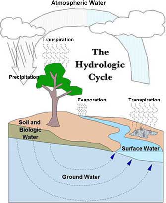
The Hydrologic Cycle
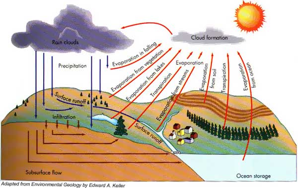
What is the Hydrologic Cycle?
The hydrologic cycle is a description of the generic reservoirs or forms that water resides in and on the earth, the interconnections between these reservoirs, and how water in its various forms moves between the reservoirs.
The world's water is in constant motion, flowing downhill by gravity, pumped into the atmosphere by evaporation fueled by Sun's heat, and returned as rain and snow. Except for the oceans, most of it moves underground. The hydrologic cycle is a simple way to represent this motion. Water at the surface (wetlands, lakes, rivers, oceans) evaporates into the atmosphere, leaving impurities behind. Moisture moves around the globe with the weather patterns, and rain and snow condense from it. Some of this precipitation runs back to surface water bodies and some percolates into the ground to become soil moisture. Micro-organisms are constantly purifying this water as it moves in streams, wetlands, and soil. Plants transpire some of this back to the atmosphere, and some continues to percolate down to the water table where it becomes ground water. Ground water flows slowly through the earth, and eventually returns to surface water bodies or to the oceans to start the cycle all over.
The hydrologic cycle comprises different reservoirs of water: the moisture in the atmosphere at any moment (<0.01% of earth's total water), water in plant and animal tissue (<0.01%), as lakes, rivers, and wetlands (<0.03%), locked in polar ice caps and glaciers (2%), as underground water (4%), and in the oceans and seas (94%) [source: R.A. Freeze and J.A. Cherry, Groundwater, Prentice Hall, 1979].
Water may move rapidly between these reservoirs in the space of minutes or days (for example: plant transpiration, evaporation of rainwater from puddles, the moisture in storm fronts) or it may reside in storage for hundreds, thousands, or even millions of years (for example: water in large lakes, in the oceans, and in deep aquifers).
Almost all parts of the hydrologic cycle are interconnected: for example, the atmosphere and surface water reservoirs are directly interconnected via precipitation, evaporation and plant transpiration; some of the water that infiltrates into the ground returns relatively quickly to the atmosphere via transpiration and evaporation; surface waters can infiltrate into the ground to become ground water or can be fed by ground water (e.g. Batiste Springs, Lava Hot Springs, the middle Snake River).
Because of these interconnections (both natural and manmade), conflicts can arise, for example between users of surface water and ground water. In some cases, ground water extraction from shallow aquifers that naturally discharges into rivers and sustains streamflow in drought years may be responsible for decreased stream flows and inadequate flows for surface water users. Human intervention in the hydrologic cycle can cause similar and related problems. For example, diversions of river water for flood irrigation have had a major impact on local ground water tables, by replenishing aquifers locally by leakage from canals and irrigated fields; as flood irrigation has given way to sprinkler irrigation over recent decades, artificial replenishment from flood irrigation has waned, ground water levels have declined, and conflicts have arisen.
Global Water Source & Volume
| Water source | Water volume | Percent of | ||
| (in cubic miles) | total water | |||
| Oceans | 317,000,000 | 97.24% | ||
| Icecaps, glaciers | 7,000,000 | 2.14% | ||
| Groundwater | 2,000,000 | 0.61% | ||
| Fresh-water lakes | 30,000 | 0.009% | ||
| Inland seas | 25,000 | 0.008% | ||
| Soil moisture | 16,000 | 0.005% | ||
| Atmosphere | 3,100 | 0.001% | ||
| Rivers | 300 | 0.0001% | ||
| Total water volume | 326,000,000 | 100% |
Water Chemistry
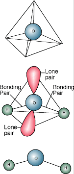 You probably know water's chemical description is H2O. A water molecule consists of one atom of oxygen bound to two atoms of hydrogen. The hydrogen atoms are "attached" to one side of the oxygen atom, resulting in a water molecule having a positive charge on the side where the hydrogen atoms are and a negative charge on the other side, where the oxygen atom is. Since opposite electrical charges attract, water molecules tend to attract each other, making water kind of "sticky." The side with the hydrogen atoms (positive charge) attracts the oxygen side (negative charge) of a different water molecule.
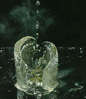
All these water molecules attracting each other mean they tend to clump together. This is why water drops are, in fact, drops! If is wasn't for some of Earth's forces, such as gravity, a drop of water would be ball shaped -- a perfect sphere. Even if it doesn't form a perfect sphere on Earth, we should be happy water is sticky.
Water is called the "universal solvent" because it dissolves more substances than any other liquid. This means that wherever water goes, either through the ground or through our bodies, it takes along valuable chemicals, minerals, and nutrients.
Pure water has a neutral pH. Pure water has a pH, of about 7, which is neither acidic nor basic.
Water's Physical Properties:
Water is unique in that it is the only natural substance that is found in all three states -- liquid, solid (ice), and gas (steam) -- at the temperatures normally found on Earth. Earth's water is constantly interacting, changing, and in movement.
 Water freezes at 32° Fahrenheit (F) and boils at 212° F. In fact, water's freezing and boiling points are the baseline with which temperature is measured: 0° on the Celsius scale is water's freezing point, and 100° is water's boiling point. Water is unusual in that the solid form, ice, is less dense than the liquid form, which is why ice floats.
Water has a high specific heat index. This means that water can absorb a lot of heat before it begins to get hot. This is why water is valuable to industries and in your car's radiator as a coolant. The high specific heat index of water also helps regulate the rate at which air changes temperature, which is why the temperature change between seasons is gradual rather than sudden, especially near the oceans.
Water has a very high surface tension. In other words, water is sticky and elastic, and tends to clump together in drops rather than spread out in a thin film. Surface tension is responsible for capillary action, which allows water (and its dissolved substances) to move through the roots of plants and through the tiny blood vessels in our bodies.
Water temperature:
Water temperature is not only important to swimmers and fisherman, but also to industries and even fish and algae. A lot of water is used for cooling purposes in power plants that generate electricity. They need cool water to start with, and they generally release warmer water back to the environment. The temperature of the released water can affect downstream habitats. Temperature also can affect the ability of water to hold oxygen as well as the ability of organisms to resist certain pollutants.
pH:
pH is a measure of how acidic/basic water is. The range goes from 0 - 14, with 7 being neutral. pHs of less than 7 indicate acidity, whereas a pH of greater than 7 indicates a base. pH is really a measure of the relative amount of free hydrogen and hydroxyl ions in the water. Water that has more free hydrogen ions is acidic, whereas water that has more free hydroxyl ions is basic. Since pH can be affected by chemicals in the water, pH is an important indicator of water that is changing chemically. pH is reported in "logarithmic units," like the Richter scale, which measures earthquakes. Each number represents a 10-fold change in the acidity/basicness of the water. Water with a pH of 5 is ten times more acidic than water having a pH of six.
Pollution can change a water's pH, which in turn can harm animals and plants living in the water. For instance, water coming out of an abandoned coal mine can have a pH of 2, which is very acidic and would definitely affect any fish crazy enough to try to live in it! By using the logarithm scale, this mine-drainage water would be 100,000 times more acidic than neutral water -- so stay out of abandoned mines.
Specific Conductance:
Specific conductance is a measure of the ability of water to conduct an electrical current. It is highly dependent on the amount of dissolved solids (such as salt) in the water. Pure water, such as distilled water, will have a very low specific conductance, and sea water will have a high specific conductance. Rainwater often dissolves airborne gasses and airborne dust while it is in the air, and thus often has a higher specific conductance than distilled water. Specific conductance is an important water-quality measurement because it gives a good idea of the amount of dissolved material in the water.
Probably in school you've done the experiment where you hook up a battery to a light bulb and run two wires from the battery into a beaker of water. When the wires are put into a beaker of distilled water, the light will not light. But, the bulb does light up when the beaker contains salt water (saline). In the saline water, the salt has dissolved, releasing free electrons, and the water will conduct an electrical current.
Turbidity:
Turbidity is a measure of the cloudiness of water. It is measured by passing a beam of light through the water and seeing how much is reflected off particles in the water. Water cloudiness is caused by material, such as dirt and residue from leaves, that is suspended (floating) in the water. Crystal-clear water, such as Lake Tahoe (where they work hard to keep sediment from washing into the lake) has a very low turbidity. But look at a river after a storm -- it is probably brown. You're seeing all of the suspended soil in the water. Lucky for us, the materials that cause turbidity in our drinking water either settle out or are filtered before the water arrives in our drinking glass at home. Turbidity is measured in nephelometric turbidity units (NTU).
Dissolved Oxygen:
Although water molecules contain an oxygen atom, this oxygen is not what is needed by aquatic organisms living in our natural waters. A small amount of oxygen, up to about ten molecules of oxygen per million of water, is actually dissolved in water. This dissolved oxygen is breathed by fish and zooplankton and is needed by them to survive.
Rapidly moving water, such as in a mountain stream or large river, tends to contain a lot of dissolved oxygen, while stagnant water contains little. The process where bacteria in water helps organic matter, such as that which comes from a sewage-treatment plant, decay consumes oxygen. Thus, excess organic material in our lakes and rivers can cause an oxygen-deficient situation to occur. Aquatic life can have a hard time in stagnant water that has a lot of rotting, organic material in it, especially in summer, when dissolved-oxygen levels are at a seasonal low.
Hardness:
The amount of dissolved calcium and magnesium in water determines its "hardness." Water hardness varies throughout the United States. If you live in an area where the water is "soft," then you may never have even heard of water hardness. But, if you live in Florida, New Mexico, Arizona, Utah, Wyoming, Nebraska, South Dakota, Iowa, Wisconsin, or Indiana, where the water is relatively hard, you may notice that it is difficult to get a lather up when washing your hands or clothes. And, industries in your area might have to spend money to soften their water, as hard water can damage equipment. Hard water can even shorten the life of fabrics and clothes! Does this mean that students who live in areas with hard water keep up with the latest fashions since their clothes wear out faster?
Suspended Sediment:
Suspended sediment is the amount of soil moving along in a stream. It is highly dependent on the speed of the water flow, as fast-flowing water can pick up and suspend more soil than calm water. During storms, soil is washed from the stream banks into the stream. The amount that washes into a stream depends on the type of land in the river's drainage basin and the vegetation surrounding the river.
If land is disturbed along a stream and protection measures are not taken, then excess sediment can harm the water quality of a stream. You've probably seen those short, plastic fences that builders put up on the edges of the property they are developing. These silt fences are supposed to trap sediment during a rainstorm and keep it from washing into a stream, as excess sediment can harm the creeks, rivers, lakes, and reservoirs.
Sediment coming into a reservoir is always a concern; once it enters it cannot get out - most of it will settle to the bottom. Reservoirs can "silt in" if too much sediment enters them. The volume of the reservoir is reduced, resulting in less area for boating, fishing, and recreation, as well as reducing the power-generation capability of the power plant in the dam.
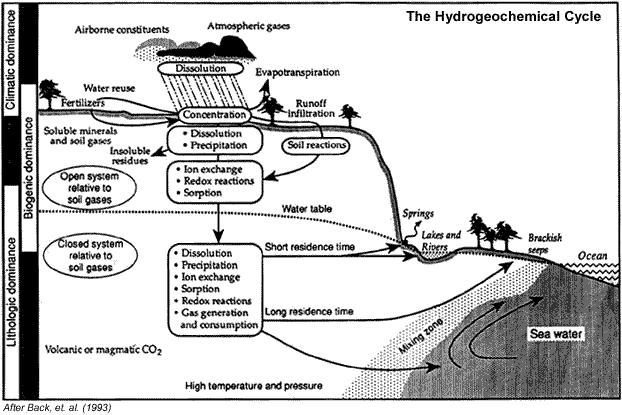
Aqueous Solution Geochemistry:
Look at a diagram of the hydrogeochemical cycle.
- Acid = substance containing hydrogen which gives free hydrogen (H + ) when dissolved in water
- Base = substance containing the OH group that yields free (OH - ) when dissolved in water
-
An acid solution is one containing an excess of free H + , and a base is one containing excess of free OH - . A reaction between an acid and a base is usually called neutralization.
For example:
-
HCl (acid) + NaOH (base) ==> H 2 O + NaCl
which are dissociated into ions:
H + + Cl - + Na + + OH - ==> H 2 O + Na + + Cl - - i.e. Na + and Cl - are unaffected.
- pH = inverse log of the concentration (activity) of free H + , or pH = -log [H + ]
-
Water dissociates into H + and OH - ;
-
the dissociation constant is: K water = [H + ] [OH - ] =10 -14
- So there has to be 10 -7 moles each of H+ and OH - in a kilogram of neutral solution at standard temperature of 25°C. One mole is 6.023 x 10 23 atoms (or molecules) and H 2 O has a molecular weight of 18 grams per mole. One kilogram of water has about 1000/18 = 55.6 moles of water or about 3.35 x 10 25 atoms of oxygen and about twice that number (6.7 x 10 25 atoms) of H + (the amount of free H + or free OH - is relatively small compared to the amount of undissociated H 2 O).
- pH ranges at 25°C from 0 to 14; pH < 7 = acidic solution; pH > 7 = basic solution. If HCl or another acid is added then pH decreases; if NaOH or another base is added then pH increases.
- pH increases as carbonic acid (a weak acid) dissociates: When carbon dioxide combines with water, such as what happens in the atmosphere when fossil fuels are burned, carbonic acid is formed: H 2 O + CO 2 ==> H 2 CO 3 . Free H + are made available during successive dissociations:
-
H 2 CO 3 ==> H + + HCO 3- carbonic acid to bicarbonate, occurs at pH ~6.4
-
HCO 3 ==> H + + CO 32- bicarbonate to carbonate, occurs at pH ~10.3
Remember, free H + is available only when acidic, or when pH < ~7. The dissociation of bicarbonate to carbonate occurs when there is too much OH - in the system and H + is "released" to balance out the base.
- Dissolved Cations and Anions in Water
Cations = electron donors, positively charged: Na + , K + , Mg ++ , Ca ++ , Fe ++ or Fe +++ , Mn ++ , Al +++
Anions = electron acceptors, neg. charged: Cl - , F - , I - , Br - , SO 4-- , CO 3-- , HCO 3- , NO 3-- , NO 2-
Metals = act like cations mostly: Cu, Zn, Pb, Co, Ni, Cr, As, Se, Mo, etc.
- Water Analyses - Need to have cation-anion balance
millequivalent (MEQ) = mole equivalent charge or anion or cation, measure of total charge due to the ion in question dissolved in the solution. Start with concentration, divide by mole wt., multiply by charge: XX mg/L / MW x CHG = MEQ
Example: NaCl in solution, Na = 50 mg/L (50 ppm): 50/23 x 1 = 2.17 MEQ
Cl = 77 mg/L (77 ppm): 77/35.5 x -1 = -2.17 MEQ
So, if the total cation and anion MEQ’s are not balanced, some error exists in the analysis.
¨ Number Of Lakes ------------------------------------------- More Than 2,000
¨ Largest Lake -- Pend Oreille -------------------------------- 148 Square Miles
¨ Deepest Lake -- Pend Oreille ------------------------------- More Than 1,100 Feet
¨ Highest Waterfall--------------------- 600 feet, Big Fiddler Creek, Boise River Basin
¨ Miles Of Streams and Rivers -------------------------------- 93,000 Miles
¨ Longest River -- Snake River ------------------------------- 779 Miles
¨ Average Annual Precipitation --------Varies From Less than 10 to More than 60 Inches
¨ Most Precipitation in 24-Hour Period----- 7.7" of rain, Rattlesnake Creek, Idaho, 1909
¨ Annual Stream Inflow to State ------------------------------ About 37 Million Acre-feet
¨ Annual Stream Outflow to State----------------------------- About 75 Million Acre-feet
¨ Irrigated Area of State -------------------------------------- 4 Million Acres
¨ Highest Dam----------------------------- Dworshak, North Fork Clearwater, 717 feet.
¨ Active Reservoir Storage Capacity ------------------------- 12,384,000 Acre-feet
¨ Largest Active Storage Reservoir -- Dworshak ------------- 2,016,000 acre-feet
¨ Snake Plain Aquifer Storage -- Top 100 Feet of Aquifer -- About 100 Million Acre-feet
What is Surface Water?
Water is continually moving around, through, and above the Earth. It moves as water vapor, liquid water, and ice. It is constantly changing its form. Water on Earth is known by different terms, depending on where it is and where it came from.
* Meteoric water - is water in circulation
* Connate water - "fossil" water, often saline.
* Juvenile water - water that comes from the interior of the earth.
* Surface water - water in rivers, lakes, oceans and so on.
* Subsurface water - Groundwater, connate water, soil, capillary water
* Groundwater - exists in the zone of saturation, and may be fresh or saline.
The movement of water is referred to as the global water cycle (hydrologic cycle). Precipitation, evaporation/transpiration, and runoff (surface runoff and subsurface infiltration) are the primary phases in the hydrologic cycle. The global water budget is based on the recycling (movement, storage, and transfer) of the Earth’s water supply.
The direct process by which water changes from a liquid state to a vapor state is called evaporation. In transpiration, water passes from liquid to vapor through plant metabolism. Plants are classified as hydrophytes, phreatophytes, mesophytes, or xerophytes. Hydrophytes take their nutrients directly from the water. Mesophytes are plants that grow under well-balanced moisture supplies. Xerophytes are plants that are adapted to dry conditions. Phreatophytes are long rooted plants that absorb water from the water table or directly above it. Golden tamarisk and mesquite are phreatophytes.
How Much Water is There In and On the Earth?
The volume of the Earth’s water supply is about 326 million cubic miles. Each cubic mile is greater than 1 trillion gallons. Although water is abundant on a global scale, more than 99% is unavailable for our use. A mere 0.3% is usable by humans, with an even smaller amount accessible! The oceans, ice caps, and glaciers contain most of the Earth’s water supplies. Ocean water is too saline to be economically useful, while glaciers and icecaps are "inconveniently located."
Surface water supplies, primarily river runoff, are about 300 cubic miles. That means we have about 1/10,000th of 1% to use! Conservation is important!
Surface runoff plays an important role in the recycling process. Not only does it replenish lakes, streams, and groundwater; it also creates the landscape by eroding topography and transporting the material elsewhere.
A stream typically transports three types of sediment- dissolved load, suspended load, and bed load. Chemical weathering of rocks produces ions in solution (examples- Ca2+, Mg+, and HCO3+). Hence, a dissolved load. High concentrations of Ca2+ and Mg+ are also known by another name - hard water. Some of you may be very familiar with hard water!
Suspended sediment makes water look cloudy or opaque. The greater the suspended load, the muddier the water. Bed load (silt- to boulder-sized, but mostly sand and gravel) settles on the bottom of the channel. Bed load sediment moves by bouncing or rolling along the bottom. The distance that bedload travels depends on the velocity of the water.
Factors Affecting Surface Runoff
Several factors can affect surface runoff. The extent of runoff is a function (ƒ) of geology, slope, climate, precipitation, saturation, soil type, vegetation, and time. Geology includes rock and soil types and characteristics, as well as degree of weathering. Porous material (sand, gravel, and soluble rock) absorbs water far more readily than does fine-grained, dense clay or unfractured rock. Well-drained material (porous) has a lower runoff potential therefore has a lower drainage density. Poorly-drained material (non-porous) has a higher runoff potential, resulting in greater drainage density. Drainage density is a measure of the length of channel per unit area. Many channels per unit area means that more water is moving off of the surface, rather than soaking into the soil.
Drainage basins or watersheds have different shapes and sizes. Large drainage basins are usually divided into smaller ones. Size and shape have a direct effect on surface runoff. Refer to Module 3 to see information about drainage basins.
Which Type of Drainage Basin Has the Greatest Effect on Surface Runoff?
Long, narrow drainage basins generally display the most dramatic effects of surface runoff. They have straight stream channels and short tributaries. Storm waters reach the main channels far more rapidly in long narrow basins than in other types of basins. Flash floods are common in long, narrow drainage basins, resulting in greater erosion potential.
Topography (relief) and slope (gradient) are additional factors affecting water velocity, infiltration rate, and overland flow rate. Water velocity, infiltration rate and overland flow rate affect surface and subsurface runoff rates.
Climate is also important. Precipitation (type, duration, and intensity) is the key climatic factor. Infrequent torrential downpours easily erode sediment-laden topography, while soft drizzly rain infiltrates the soil.
Vegetation aids in slope stability. Removal of vegetation by fire, clear-cutting (logging), or animal grazing often results in soil erosion. The eroded material is washed into streams, adding to the sediment load.
Runoff Paths
There are three runoff paths that water follows to reach a stream channel- throughflow, overland flow, and groundwater flow.
Throughflow is a shallow subsurface flow that occurs above the groundwater table. A major requirement for throughflow is a good infiltration capacity. Throughflow commonly occurs in humid climates containing thick soil layers and good vegetation cover. In such locations, saturated soil conditions result in surface runoff (overland flow).
Overland flow occurs when precipitation exceeds infiltration rates. Overland flow is common in semi-arid regions, sparsely vegetated and/or disturbed areas, and locations containing dense, clay-rich layers.
Surface Water /Groundwater Interaction
Surface streams have an effect on the groundwater table. Influent streams recharge groundwater supplies. Influent streams, located above the groundwater table, flow in direct response to precipitation. Water percolates down through the vadose zone to the water table, forming a recharge mound.
Effluent streams are discharge zones for groundwater. Effluent streams are generally perennial (flow year round). Groundwater seeps into stream channels, maintaining water flow during dry seasons.
The Big Lost River in Idaho is a good example of an intermittent, ephemeral influent stream. Natural flow of the Big Lost River terminates in the Big Lost River Sinks, located on the INEEL. But, local irrigation now diverts the Big Lost River from its natural terminus
Groundwater supplies 30% of the water present in our streams. Recall that effluent streams act as discharge zones for groundwater during dry seasons. This phenomenon is known as base flow. Groundwater overdraft reduces the base flow, which results in the reduction of water supplied to our streams.
Equally important is water quality. Salinity, a by-product of water flowing over salt beds, salt springs, and irrigation and evaporation, increases with distance downstream.
Surface Hydrology
Idaho, known as the Potato State, could just as logically be called the river state. We have over 93,000 thousand miles of rivers, streams and creeks, in addition to 1,000s of lakes and reservoirs, and these waters are deeply connected to most Idahoans lives. We float them, fish them, swim in them, irrigate with them, and generate power with them. They have shaped the landscape of the entire state - both at normal flow levels, and when in flood stage.
How we use our riverways is an on-going issue for Idahoans. Consider these facts about how we use Idaho's rivers:
* Idaho Rivers are home to 19 species of fish that are listed as endangered, threatened, or of "special concern."
* 420,000 anglers fish on Idaho rivers annually.
* Idaho has over 3100 miles of whitewater suitable for rafting, kayaking or canoeing.
* 2000 miles of Idaho's rivers are designated as State Protected Rivers through conservation groups and citizens.
* Over 400 miles of Idaho's Rivers have minimum streamflow water rights, which help protect fish, wildlife, water quality, and recreational values.
* 577 miles of Idaho rivers are currently designated as National Wild, Scenic or Recreational Rivers.
* Idaho water produces nearly 1/3 of the US potato crop.
* There are over 232 major dams and 777 major irrigation diversions on Idaho rivers.
* Idaho hydropower generates enough electricity for 320,000 to 340,000 all-electric homes built to energy efficient standards or 175,000 built to the present state standard.
Most of Idaho's rivers and streams flow into one of 5 major river basins; the Snake, the Clearwater, the Salmon, Bear, and the St. Joe. These rivers have been important parts of Idaho history from travel routes for early explorers, to industrial, domestic, and recreational resources for today's Idahoans. In the pages of this atlas you can explore some of the natural history of the regions drained by these great rivers.
Streamflow and Precipitation
A basic understanding of units of measurement and data reporting in hydrology are required to use the data bases and coverages of Idaho hydrology and precipitation found on the Atlas. The basic unit of streamflow in the United States is cubic feet per second (cfs), or the volume of water that flows past a cross-section of a river in a second. Most of the data found here is based on the daily mean discharge, which is the average cfs for all seconds in a day. The mean annual discharge is the average of all daily mean discharges in a year. Precipitation is reported as a depth. To fully understand the data, it is useful to understand how that data is collected.
Instantaneous Streamflow Measurement
Streamflow (Q) is calculated by multiplying the velocity (V) of the water in a stream times the area (A) of the cross section:
Q=V*A
The area is simply the width (W) of the river times the depth (Y). Because depth and velocity change through any cross section (it’s faster and deeper in the center of the river), several measurements must be made. Typically, the stream gauger splits the stream into several cells and measures W, Y, and V in each cell, calculates Q in each cell, then adds up all the cells to get the total Q. The United States Geological Survey recommends 20 cells in a cross section.
The stream gauger moves across the river measuring the distance from the bank to keep track of width, and takes a depth measurement at a station. A salmon swimming upstream could tell you that the stream velocity is slower at the bottom of the river than at the top. How then do we report the velocity in a cell if it changes? Fortunately, the relationships between depth and velocity are fairly well known. The average velocity typically occurs at 60% of the depth measured from the top. So we measure the depth, then place a current meter at 0.6 times the depth to get the average velocity for that station. If the stream is shallow, the gauger will wade. More elaborate suspension systems, boats or bridges are required in deep and fast flow. Here is an example of calculating discharge from field data.
Continuous Streamflow Measurement
The above techniques give us the discharge of a stream only at the time of measurement. Does this mean that every time the river rises from a rainfall that we have to re-measure the streamflow? Yes and no. We can construct a continuous record of streamflow, called a hydrograph, from what is called a stage-discharge relationship. Stage is simply the height of the water surface relative to the height of a reference marker that doesn’t change. Stage is measured with a staff gage. The simplest staff gage is essentially a meter stick placed in the stream. When a stream gauger measures discharge, he/she records the stage. Stage is continuously monitored by charting the history of a float in a stilling well. The float moves up and down with the water level and rotates a drum on which a sheet of paper is attached. At the same time, a pen moves across the drum at a known rate. The result is a line describing the stage history. Fortunately, for any given stage in a cross section that is not altered by erosion, the discharge is always the same. Discharge is measured at several stages, then a relationship is established between stage and discharge through a mathematical equation. If stage is continuously monitored, continuous discharge can be calculated by the stage-discharge relationship.
Streamflow Hydrograph
A hydrograph is a plot of discharge against time. The time scale can be in hours, days, months, or even years. The rise and fall of discharge is the response of the watershed to inputs of precipitation. A simple storm hydrograph contains 4 components: baseflow, the rising limb, the crest, and the falling limb. The arrangement of these 4 components produce a unique shape of a hydrograph that results from a combination of properties of the storm and the watershed. For example, a hard rain on pavement will result in a very steep rising limb, and a watershed containing wetlands will usually produce hydrographs with long falling limbs as the wetlands slowly release water.
Precipitation Measurement
Precipitation is reported as a depth of water in inches, and includes rain and snow. The depth does not include the actual depth of snow, but is the depth of water that would result from melting the snow. Rainfall is measured in rain gauges which are essentially buckets that collect water. If you record the change in depth in the bucket with time you get a rainfall rate or intensity. A bar-chart of precipitation that falls in a given unit of time is called a hyetograph. Comparing a hyetograph to a hydrograph allows you to investigate how quickly streams respond to precipitation.
Running Water
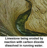
Running water is the most powerful agent of erosion. Continents are eroded primarily by running water at an average rate of 1 inch every 750 years. The velocity of a stream increases as its gradient increases but velocity is also influenced by factors such as degree of turbulence, position within the river, the course of the stream, the shape of the channel and the stream load.
River Cycles
Stages in the cycle of river erosion are labeled as youth, maturity and old age. Each stage has certain characteristics that are not necessarily related to age in years - only phases in development. Typically, rivers tend to have old-age-type development at their initial mouths and youthful development at their upper reaches. So the three stages may grade imperceptibly from one to another and also from one end of the stream to the other.
The youthful stage is characterized by rapid downcutting, high stream gradient, steep-sided valleys with narrow bottoms and waterfalls. The mature stage is characterized by a longer, smoother profile and no waterfalls or rapids.
Gradient is normally expressed as the number of feet a stream descends each mile of flow. In general, a stream's gradient decreases from its headwaters toward its mouth, resulting in a longitudinal profile concave towards the sky.
Base Level
The base level of a stream is defined as the lowest level to which a stream can erode its channel. An obstacle such as a resistant rock across a stream can create a temporary base level. For example, if a stream passes into a lake, it cannot erode below the level of the lake until the lake is destroyed. Therefore different stretches of a river may be influenced by several temporary base levels. Of course the erosive power of a stream is always influenced by the ocean which is the ultimate base level below which no stream can erode. Many streams in Idaho eventually reach the ocean through the Columbia River.
If the base level is raised in some manner such as by a landslide blocking a stream, the stream's velocity is reduced and it can no longer carry as much material. Sedimentary material will then be deposited in the lake formed by the landslide. Conversely, if the base level is lowered, the stream will begin eroding its channel downward.
Transportation of Material
Running water transports material in 3 ways: solution, suspension and by rolling and bouncing on the stream bottom. 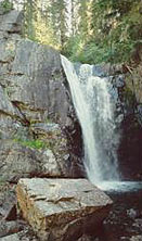 Dissolved material is carried in suspension. About 270 million tons of dissolved material is delivered yearly to the oceans from streams in the United States. Particles of clay, silt and sand are generally carried along in the turbulent current of a stream. Some particles are too large and heavy to be picked up by water currents, but may be pushed and shoved along the stream bed.
Waterfalls
Waterfalls are a fascinating and relatively rare occurrence. Waterfalls may be caused in several ways. For example, where a relatively resistant bed of rock overlies less resistant rock, undermining of the less resistant rocks can cause a falls. Waterfalls are short-lived features in the history of a stream as they are created by a temporary base level. As time passes, falls may slowly retreat upstream, perhaps as rapidly as several feet per year. There are many spectacular waterfalls in Idaho, including the 212-foot-high Shoshone Falls in the Snake River Canyon just north of Twin Falls.
What is Meant by “Surface and Ground Water Interaction”?
Aquifers exist beneath much of the land on which we live and work. Ground water occurs within the pores between soil and rock particles and in cracks and fractures in rocks. The aquifers are often partially fed by seepage from streams and lakes. In other locations, these same aquifers may discharge through seeps and springs to feed the streams, rivers, and lakes. Outstanding examples of both situations can be found in the Snake River Basin.
 |
|
Photo courtesy of the National Park Service
|
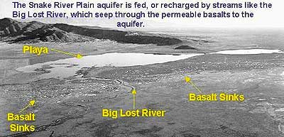
The Big Lost River is an example of a river feeding an aquifer. The river flows out of a mountain valley on the northwest margin of the Snake River Plain and entirely disappears through seepage into the permeable lava of the Plain. The underlying Snake River Plain aquifer flows to the southwest, ultimately discharging in the form of springs along the wall of the Snake River canyon.
The Snake River provides an excellent example of a river fed by ground water. As the Snake River flows across southern Idaho much of the flow is diverted for irrigation. At Shoshone Falls, about 30 miles downstream of Milner Dam, the river may nearly dry up due to irrigation diversions. In the next 40 miles downstream, the river is again “reborn” in the impressive Thousand Springs area, where springs collectively discharge more than 5,000 cubic feet per second. Niagara Springs is an example of the many scenic springs in the Thousand Springs area. These river “gains” provide the majority of the downstream flow during summer.
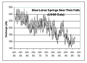 Discharges from springs are often relatively constant, but may fluctuate with the season and from year to year, depending upon natural weather patterns and man-induced effects of pumping and irrigation.
Discharge of Blue Lakes Spring along the Snake River near Twin Falls shows both seasonal and long-term variation. Much of the short and long-term variation in the flow of Blue Lakes Spring is due to distribution and application of water from the Snake River for irrigation and ground water pumping.
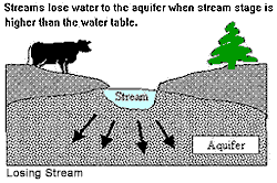
In some situations, river seepage (losses to the aquifer) may be affected by ground water pumping and natural variations in aquifer water level. When the aquifer water level is near land surface, seepage from the river is partially controlled by the height of the aquifer water level, (see losing stream illustration). Activities or events that result in a lowering of the water table, such as ground water pumping, induce more seepage from the river.
 |
 |
 |
|
Losing Stream
|
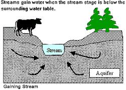
Gaining Stream
|
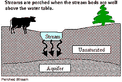
Perched Stream
|
Conversely, events that cause the aquifer water level to rise (recharge events) will result in a decrease in river seepage. If aquifer water levels rise above the level of the river, what was previously a losing river reach will become a reach that is gaining water from the aquifer.
Another hydrologic condition exists that is very important in understanding surface and ground water interaction. A surface water body is “perched” above an aquifer when aquifer water levels are well below the bed of the river, stream, or lake (see perched stream illustration). Under these conditions, water will seep from the surface water body to the ground water, but the surface water body will not be affected by aquifer water levels and consequently does not change in response to ground water pumping. Nearby ground water pumping will cause a lowering of the water table, but will not affect surface water supplies.
In summary, any of three conditions may exist that determine if, or how, ground water use may affect surface water resources. These conditions are:
1) an interconnected river (or lake) and aquifer, where the river is losing water to the aquifer,
2) an interconnected river or lake in which the river or lake is gaining water from the ground water, and
3) a perched river which is losing water to the aquifer.
In the first condition river losses will increase in response to ground water pumping. In the second condition, river gains will decrease in response to ground water pumping. In either case, ground water pumping will result in a depletion or capture of surface water. In the third case, ground water pumping has no impact on surface water resources. All these conditions may exist in the same river or lake at different locations or times of year.
What Controls the Degree of Surface and Ground Water Interaction?
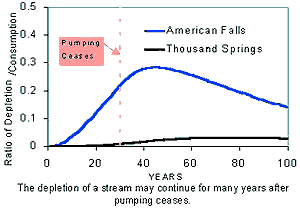 An analogy is often made between an overflowing horse trough and an aquifer. The horse trough has a continual source of water flowing in at a fixed rate. Obviously, the trough must also have an overflow that is flowing at the same rate. If a small pump is introduced into the trough and begins pumping continuously, then the overflow will soon be depleted by an amount equal to the rate of pumping. In many ground water systems, surface water supplies are ultimately depleted by an amount of water equal to volumes pumped and consumptively used. The effects of pumping on surface water sources are normally greatly attenuated relative to the horse trough analogy. The effects of pumping on surface water supplies may be distributed over years, or even decades, depending on the size and properties of the aquifer. Johnson and others (1993) demonstrates how the stream depletion effects for 30 years of continuous pumping from the Snake River Plain aquifer persist for decades after pumping ceases (see graph right).
Difficulties arise in determining the timing, location, and magnitude of the impacts. The degree to which ground water pumping depletes surface water supplies is dependent on several features of the particular basin. Considerations include: 1) the degree to which the river and aquifer are interconnected, 2) the distance between the river and the pumping source, 3) the rate of pumping, and 4) the physical characteristics of the aquifer. These factors are discussed in the following paragraphs.
The degree of river and aquifer interconnection is of great importance in controlling the amount of surface water depletion resulting from ground water pumping. If a river is perched above an aquifer, ground water pumping has no effect on river flow. If the river is not perched, but sediments have accumulated in the riverbed, or the river only slightly penetrates into the aquifer, then the hydraulic communication between the river and aquifer may be limited. Examples are shown in the following illustrations: partially penetrating river with silt deposition and fully penetrating rivers. Spring discharge will nearly always be impacted by nearby ground water pumping from the same aquifer.
 The distance between a surface water body and a pumping location strongly affects the timing and degree that pumping will impact stream depletion. Pumping near an interconnected surface water body will have a nearly immediate impact on the surface water source. The impact may be nearly equal to the rate of ground water pumping. At greater distances, the effects of pumping will be distributed over longer time periods and may be shared with other hydraulically connected surface water bodies.
The rate of stream depletion associated with pumping from a given location is normally proportional to the rate of ground water pumping. If the rate of pumping from a given well is doubled, then the rate of stream depletion resulting from pumping that well also doubles. Stream depletion will be proportional to pumping rate unless aquifer water levels change so dramatically that springs are dried up, streams become perched, or aquifer properties change.
Ground water that is pumped, but not consumptively used (for example, industrial pumping that is discharged to seepage ponds), may return to the aquifer from which it was extracted and have little or no impact on surface or ground water supplies outside the immediate vicinity. Similarly, ground water pumped in excess of the amount required for crops to grow may return to the aquifer and have little or no quantitative impact on the surrounding resource. It is the amount of water that is permanently extracted from the aquifer and consumptively used that is of significance.
 Aquifer physical characteristics also affect the timing and magnitude of stream depletion from pumping. Aquifer layering, water transmission, and storage properties may have a strong influence on the direction and rate of propagation of pumping effects. Wells completed in deeper layers may have a more disbursed and delayed impact on surface water bodies than wells completed in upper layers of an aquifer. Highly transmissive aquifers with limited water storage capacity will transmit effects more rapidly than aquifers of lower permeability or higher storage capacity.
A common misconception is that impacts of ground water pumping may be projected along estimated flow paths through an aquifer. If this were true, then only down-gradient streams and springs would be affected by up-gradient pumping. In fact, the effects of ground water pumping propagate radially in all directions (assuming aquifer properties are uniform), regardless of the direction of ground water flow. This means that pumping effects are felt upstream, laterally across the gradient, and downstream, making conjunctive water rights allocation extremely difficult. In the case of the Snake River Plain aqufier, this means that even down-gradient pumpers have some impact on the upper river reaches.
How Can Pumping Impacts be Measured or Estimated?
Measurement of the stream and spring depletion from ground water pumping requires controlled testing in the field. The well of interest is turned on for a period of relatively continuous pumping. The effects on a spring or stream are then determined by measuring changes in the flow of the spring or stream. This obviously requires that interference from other wells or recharge activities be minimized during the test period.
The impacts of ground water pumping on surface water bodies can be measured in relatively few situations. Measurable impacts require situations where there is little interference from other wells, close proximity of the pumping location and the surface water, and a pumping rate that is a measurable proportion of stream or spring discharge. If nearby wells exist that have a capacity similar to that of the well of interest, and these wells are operating, it becomes difficult or impossible to isolate the effects of a single well on a nearby spring or stream. If the well of interest is a great distance from the spring or stream (perhaps a few miles or more), the effects may be so greatly attenuated that testing becomes infeasible. If the pumping rate is small relative to the discharge of the stream or spring, then changes in the spring or stream flow may be immeasurably small. Any of these conditions make the measurement of depletion due to pumping impracticable and require that theoretical methods be employed.
Ground water flow theory can be applied to estimate spring or stream depletion in several ways. Some of the most simple techniques were developed by Jenkins (1968) and Glover (1968). These methods use an analytical equation to calculate graphs that generically relate pumping to depletion. Depletion rates are a function of aquifer transmissivity and storativity and the distance between the stream and well. The depletion is assumed to be proportional to the pumping rate. Application of these methods involves numerous simplifying assumptions including: 1) the aquifer is infinite except where cut by the stream, 2) the stream fully penetrates the aquifer, 3) the aquifer characteristics are uniform, 4) the stream is approximately straight, and 5) aquifer thickness is not significantly changed by pumping. When these assumptions are too restrictive, more sophisticated methods must be employed.
Numerical modeling of stream depletion avoids many of the assumptions required in the more simple analytical techniques. Numerical modeling allows us to incorporate all of our understanding (which may be incomplete or flawed) of the real system into the process of calculating depletion. The sophistication of the model should be commensurate with the level of our understanding of the real system. Simple numerical models supported by limited data may still give more accurate estimates than the described analytical methods. Numerical modeling, however, does require more effort than application of the analytical techniques. In cases where entire aquifers are considered, and multiple reaches of streams are interconnected with the aquifer, the modeling process may become very complicated.
In some cases, the results of numerical models may be generically represented by response functions or coefficients. The response functions are determined from numerical models and quantify the relationship between pumping and stream depletion for specific pumping locations and stream reaches. Response functions are being determined to relate depletion of surface flows of the Snake River due to ground water pumping of the Snake River Plain aquifer.
How do Surface Water Bodies Respond to Aquifer Recharge?
The previous discussion has focused on the impacts of ground water pumping on stream and spring discharge. There is an equal and opposite effect for conditions of aquifer recharge on spring and river flow. As ground water pumping serves to deplete stream flow, aquifer recharge enhances stream flow. All of the previous discussion related to pumping also relates to recharge.
What is an Aquifer?
An aquifer is a body of saturated rock through which water can easily move. Aquifers must be both permeable and porous and include such rock types as sandstone, conglomerate, fractured limestone and unconsolidated sand and gravel. Fractured volcanic rocks such as columnar basalts also make good aquifers. The rubble zones between volcanic flows are generally both porous and permeable and make excellent aquifers. In order for a well to be productive, it must be drilled into an aquifer. Rocks such as granite and schist are generally poor aquifers because they have a very low porosity. However, if these rocks are highly fractured, they make good aquifers. A well is a hole drilled into the ground to penetrate an aquifer. Normally such water must be pumped to the surface. If water is pumped from a well faster than it is replenished, the water table is lowered and the well may go dry. When water is pumped from a well, the water table is generally lowered into a cone of depression at the well. Groundwater normally flows down the slope of the water table towards the well.
One of Idaho's major aquifers is the Snake River Plain Aquifer.
Is an Aquifer an Underground River?
No. Almost all aquifers are not rivers. Since water moves slowly through pore spaces in an aquifer's rock or sediment, the only life-forms that could enjoy floating such a 'river' would be bacteria or viruses which are small enough to fit through the pore spaces. True underground rivers are found only in cavernous rock formations where the rock surrounding cracks or fractures has been dissolved away to leave open channels through which water can move very rapidly, like a river.
Ground water has to squeeze through pore spaces of rock and sediment to move through an aquifer (the porosity of such aquifers make them good filters for natural purification. Because it takes effort to force water through tiny pores, ground water loses energy as it flows, leading to a decrease in hydraulic head in the direction of flow. Larger pore spaces usually have higher permeability, produce less energy loss, and therefore allow water to move more rapidly. For this reason, ground water can move rapidly over large distances in aquifers whose pore spaces are large (like the lower Portneuf River aquifer) or where porosity arises from interconnected fractures. Ground water moves very rapidly in fractured rock aquifers like the basalts of the eastern Snake River Plain. In such cases, the spread of contaminants can be difficult or impossible to prevent.
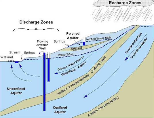
What does an aquifer look like?
Every aquifer is unique, although some are more generic than others. The boundaries of an aquifer are usually gradational into other aquifers, so that an aquifer can be part of an aquifer system. The top of an unconfined aquifer is the water table. A confined aquifer has at least one aquitard at its top and, if it is stacked with others, an aquitard at its base.
 |
The diagram represents a cut-away perspective view of this system of multiple aquifers and is greatly exaggerated in its vertical scale to show some of the details. Several different aquifers occur in this valley. In the northern valley (beneath Chubbuck and north Pocatello) multiple confined aquifers are stacked on top of one another and separated by aquitards made of clay; the aquifers tapped by Chubbuck's municipal wells are in the fractured basalts of the eastern Snake River Plain. In the southern valley (Portneuf Gap to Red Hill) the upper surface of the unconfined aquifer is the water table.
How Does an Aquifer Work?
An aquifer is filled with moving water and the amount of water in storage in the aquifer can vary from season to season and year to year. Ground water may flow through an aquifer at a rate of 50 feet per year or 50 inches per century, depending on the permeability. But no matter how fast or slow, water will eventually discharge or leave an aquifer and must be replaced by new water to replenish or recharge the aquifer. Thus, every aquifer has a recharge zone or zones and a discharge zone or zones.
Recharge zones are typically at higher altitudes but can occur wherever water enters an aquifer, such as from rain, snowmelt, river and reservoir leakage, or from irrigation. Discharge zones can occur anywhere; in the diagram, discharge occurs not only in springs near the stream and in wetlands at low altitude, and also from wells and high-altitude springs.
The amount of water in storage in an aquifer is reflected in the elevation of its water table. If the rate of recharge is less than the natural discharge rate plus well production, the water table will decline and the aquifer's storage will decrease. A perched aquifer's water table is usually highly sensitive to the amount of seasonal recharge so a perched aquifer typically can go dry in summers or during drought years.
Why is Groundwater So Clean?
Aquifers are natural filters that trap sediment and other particles (like bacteria) and provide natural purification of the ground water flowing through them.
Like a coffee filter, the pore spaces in an aquifer's rock or sediment purify ground water of particulate matter (the 'coffee grounds') but not of dissolved substances (the 'coffee'). Also, like any filter, if the pore sizes are too large, particles like bacteria can get through. This can be a problem in aquifers in fractured rock (like the Snake River Plain, or areas outside the sediment-filled valleys of southeast Idaho).
Clay particles and other mineral surfaces in an aquifer also can trap dissolved substances or at least slow them down so they don't move as fast as water percolating through the aquifer.
Natural filtration in soils is very important in recharge areas and in irrigated areas above unconfined aquifers, where water applied at the surface can percolate through the soil to the water table. For example, in the lower Portneuf River valley, a protective layer of silt in the southern valley provides natural protection to the aquifer from septic systems, pesticide application, and accidental chemical spills.
Despite natural purification, concentrations of some elements in ground water can be high in instances where the rocks and minerals of an aquifer contribute high concentrations of certain elements. In some cases, such as iron staining, health impacts due to high concentrations of dissolved iron are not a problem as much as the aesthetic quality of the drinking water supply. In other cases, where elements such as fluoride, uranium, or arsenic occur naturally in high concentrations, human health may be affected.
How is an Aquifer Contaminated?
Contaminants reach the water table by any natural or manmade pathway along which water can flow from the surface to the aquifer.
Deliberate disposal of waste at point sources such as landfills, septic tanks, injection wells and storm drain wells can have an impact on the quality of ground water in an aquifer.
 |
In general, any activity which creates a pathway that speeds the rate at which water can move from the surface to the water table has an impact. Waste water leaking down the casing of a poorly constructed well bypasses the natural purification afforded by soil. Excessive addition of fertilizer, agrichemicals, and road de-icing chemicals over broad areas, coupled with the enhanced recharge from crops, golf courses and other irrigated land and along road ditches, are common reasons for contamination arising from non-point sources. Removal of soil in excavations and mining reduces the purification potential and also enhances recharge; in some cases, such as the Highway Pond gravel pits south of Pocatello, the water table is exposed and becomes directly vulnerable to the entry of contaminants.
What is Groundwater?
 |
|
figure 1. Click on image for larger view.
|
Groundwater is the water that lies below the surface of the ground and fills the pore space as well as cracks and other openings. Porosity is the percentage of a rock's volume that is taken up by openings. Most sedimentary rocks such as sandstone, shale and limestone can hold a large percentage of water. Loose sand may have a porosity of up to 40 percent; however, this may be reduced by half as a result of recrystallization and cementation. Even though a rock has high porosity, water may not be able to pass through it. Permeability is the capacity of a rock to transmit a fluid such as water. For a rock to be permeable, the openings must be interconnected. Rocks such as sandstone and conglomerate have a high porosity because they have the capacity to hold much water.
To understand porosity versus permeability, visualise that a sponge is both porus and permeable- meaning that it can both hold and transmit water. Styrofoam is an example of a material that is very porous, but lacks porosity. Thus styrofoam, though spongy, does not absorb or transmit water.
Why is Groundwater so Important?
Ground water is the second largest reservoir of water in the hydrologic cycle. But more importantly, it is the predominant source of drinking water in many western states. For example, ground water provides more than 95% of the drinking water used in Idaho.
The amount of ground water used in southeast Idaho, alone, was more than 800 million gallons per day. Of this, over 90% was used for agricultural purposes.
What is the Water Table?
 In response to gravity, water seeps into the ground and moves downward until the rock is no longer permeable. The subsurface zone in which all openings of the rock are filled with water is called the zone of saturation. The upper surface of the zone of saturation is called the water table. The zone that exists between the water table and the ground surface is called the zone of aeration. In order to be successful, a well must be drilled into the zone of saturation. The velocity at which water flows underground depends on the permeability of the rock or how large and well connected the openings are.
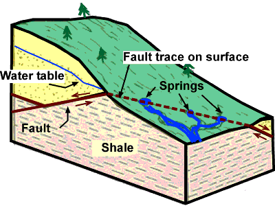
Springs occur where water flows naturally from rock onto the surface of the land. Springs may seep from places where the water table intersects the land surface. Water may also flow out of the ground along fractures.
Why Do Some "Artesian" Wells Flow?
 |
Wells that are drilled into confined aquifers can flow naturally under the higher pressure created by ground water trapped beneath confining layers.
The artesian well shown is a special kind of artesian well because it is a flowing artesian well. Like a pipe full of water, the confined aquifer into which this well is drilled sustains higher water pressure than in the unconfined aquifer above it, so that water is forced to rise higher in the artesian well than the local water table around it. If the water level rises above the top of the well, the well flows under natural water pressure.
Groundwater Resources
Idaho relies heavily on underground water supplies for agricultural, domestic and industrial uses. Groundwater is the largest reservoir of fresh water on the earth and is the predominant source of drinking water in many western states.
In 1995, groundwater provided more than 95% of Idaho’s drinking water from private and municipal wells. The amount of groundwater used in southeast Idaho, alone, was more than 800 million gallons per day.
Part of Idaho’s groundwater resource includes geothermal groundwater, or water naturally heated within the earth’s crust, that is available at or near the surface, either through wells or in natural springs.
Idaho has the third highest number of geothermal springs in the continental U.S.: some 258 active springs, with average water temperature of about 120° F, and individually as high as 203° F.
Idaho also has more than 600 geothermal water wells which provide heated water for recreation, aquaculture, and heating. Idaho's state capital building is heated with geothermal water, and Boise’s Warm Springs Avenue was the first geothermal heating district in The United States.
Areas of porous rock and sediment which hold water and give it up easily enough to provide water for a beneficial use are called aquifers (for drinking water and other non-thermal supplies). Where the water is heated geothermally, the groundwater resource is usually termed a geothermal reservoir.
Ground water issues forth in springs where water flows naturally from rock onto the surface of the land. Springs may seep from places where the water table intersects the land surface. Water may also flow out of the ground along fractures.
In most cases these springs contain water that has fallen upslope, been absorbed into the ground, and spent a few weeks to thousands of years traveling to the point of issue (the average amount of time spent in an aquifer by a water molecule called residence time).
Although most irrigation water today is provided from surface sources and wells, many an early homestead was located next to a spring.
Idaho has numerous aquifers which comprise an essential part of the state's overall water supply.
Unconsolidated aquifers hold water in pore spaces between the grains of sand and gravel in loose sediment, and are commonly known as valley-fill aquifers (e.g. The Rathdrum Prairie, Payette River valley, and lower Portneuf River valley).
Those which hold water in the cracks and pore spaces of solid rock are classified as consolidated aquifers. Idaho has two major types of consolidated aquifers: those in basalt (e.g. the Eastern Snake River Plain and Clearwater Plateau), and those in other volcanic and sedimentary materials that have been compacted and solidified. The amount of water available in these consolidated aquifers usually depends upon the size, number, and interconnection of cracks in the rock.
Sedimentary/volcanic aquifers in Idaho contain a mixture of unconsolidated sedimentary material, sedimentary rock (sandstone and shale), and basalt (e.g. The Treasure Valley, Salmon Falls/Rock Creek).
The most famous aquifer in Idaho is that of the Snake River Plain, which controls the economy of much of southern Idaho north and west of Pocatello (Stearns and others, 1938). Three million acres of farmland on the Snake River Plain are irrigated, with about 1/3 of this from wells and the rest from canals. This extensive irrigation system is the primary reason that Idaho has the highest per capita water consumption in the U.S.
The Snake River aquifer is a complex system, with multiple layers of high permeability. It discharges 8 million acre feet of water per year in the famous Thousand Springs area on the north wall of the Snake River canyon from Twin Falls to Hagerman. Most of the commercially produced trout in the United States are grown there.
The Snake River Plain is underlain by fractured and rubbly basalt lava flows, which form a highly permeable aquifer. Interbeds between the basalt layers are mainly sand, silt and clay, with smaller amounts of volcanic ash. Within basalts, permeable zones are mainly the tops and bottoms of lava flows, with columnar jointing in between providing slower vertical transmission of water. Rhyolite that underlies the basalt does not have high permeability, as many of the pore spaces are filled with chemical precipitates.
Water which falls mainly as snow in the mountains north and east of the eastern Snake River Plain is absorbed into the basalt in many places along the northern margin of the plain. The most obvious is the Sinks of the Big Lost River east of Howe, where waters of the Big and Little Lost Rivers, and Birch Creek sink into the lava plateau.
Dams were put on the Snake River at Milner, Minidoka, and American Falls in the early 1900s. The extensive irrigation essentially recycles the Snake River water, drawing it out of the river, and returning it to the river or the aquifer downstream. When the amount of irrigation on the Snake River Plain is reduced, output from the springs goes down also. The level of the aquifer rose dramatically after initiation of irrigation, but the level stabilized after a new equilibrium was reached. In the last 25 years, the level has begun to fall slowly.
Fundamentally, the Snake River Plain Aquifer is so large, with so much water running through it, and with residence times on the order of 100s of years, that it will be hard for man's efforts to change it much. Point sources of pollution certainly exist, but the dilution factor prevents them from becoming regional problems.
Water quality of the Snake River Plain aquifer is adversely affected by several human activities, most importantly agriculture. Runoff from fertilizer, feedlots, and potato processing plants has produced local acute pollution of the aquifer.
Another potential source of pollution is the Idaho National Engineering and Environmental Laboratory. Voluminous and expensive monitoring programs are being conducted to determine the extent of INEEL-caused pollution. The bottom line appears to be that the dry climate on the Snake River Plain combined with the huge volume of water in the Snake River Plain aquifer act to limit the amount of radionuclides that have reached the aquifer and then to dilute them below detection limits.
Idaho’s major aquifers have been prioritized based on their vulnerability to pollution by the Idaho Department of Health and Welfare, the Idaho Division of Environmental Quality, and the Idaho Department of Water Resources. Aquifers are vulnerable where groundwater is shallow or where soils are thin or very permeable. Also, the potential for contamination is greater where considerable water is applied to the land surface from precipitation or irrigation water and where population density and intensity of groundwater use are greatest.
Response Functions - What are they?
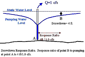 When an aquifer is pumped, ground water levels in the vicinity of the well decline, creating a cone of depression around the well. This cone of depression is the response of the system (the aquifer) to the pumping that has been introduced (see illustration right). Aquifer drawdown varies with distance from the well; consequently, the system response is location-dependent. The longer the well is pumped, the greater the drawdown becomes, making the system response time-dependent as well. If we select a specific location within the cone of depression, and by field measurements or theoretical means we quantify how drawdown varies with time in response to pumping, we have developed a simple response function for that particular location and well. In most cases, the drawdown will be proportional to the discharge of the well, so our response function, if expressed as a ratio of drawdown to well discharge, can be used to predict the system response to any pumping rate. Cones of depression from multiple pumping wells normally can be superimposed, assuming that the system response is independent of other events occurring simultaneously. These are the basic concepts of a response function.
Response functions are a means by which we can express cause and effect relationships for an aquifer or a river-aquifer system. The functions may be thought of as a series of values or ratios that express the response at a specific location to aquifer recharge or discharge at another location. Since the response changes with time, a different value is required not only for each pair of locations, but also for each time period of interest. The following two examples illustrate the concept of response functions for a) drawdown in an aquifer, and b) for depletion of a stream.
EXAMPLE 1: AQUIFER DRAWDOWN RESPONSE
Let's assume that we have two wells, A and B which are 1000 feet apart (see illustration above). We measure water levels in both wells and start pumping well A at a rate of 1.0 cubic foot per second. After 1 hour, we measure the water level in well B and note that the water level is 4 feet deeper than before we started pumping well A. The reponse ratio expressing the response of the aquifer at point B to pumping at point A would be the ratio of the drawdown at point B (4.0 feet) to the pumping rate (1cfs) at point A. In this example, the ratio 4 ft./1.0 cfs expresses the effects from pumping at one location on water levels in the aquifer at another location. It is assumed that the ratio at location B holds regardless of the pumping rate at location A. Consequently, if the pumping rate were doubled to 2 cfs, the drawdown would double to 8 feet. It must also be noted that the drawdown increases as the pumping time increases. For example, say that we continue pumping at 1 cfs and measure water levels in well B that were 6, 8 and 10 feet deeper at 2, 4 and 10 hours after we began pumping at well A, respectively. There must, therefore, be a different response ratio for each time period of interest. After one day of pumping, the ratio may have increased to 15 ft./1.0 cfs. The term response function is used to represent the series of ratios describing responses at different times.
In addition to describing the response of water levels in an aquifer to ground water pumping, response functions may be used to describe the effect of ground water pumping (or recharge) on surface water resources. When surface water resources are in hydraulic connection with an aquifer, ground water pumping or recharge can affect lake levels or flows in springs and streams. An example of a response function for a stream-aquifer system follows.
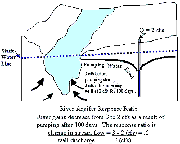 EXAMPLE 2: RIVER DEPLETION RESPONSE
Let's assume that we have a stream that traverses a plain and is in hydraulic connection with an underlying aquifer (see figure at left). That stream (a gaining stream) is being fed by the aquifer at a rate of 3 cubic feet per second (cfs) in our reach of interest between two gaging stations. A new well installation in the aquifer begins continuous pumping at a rate of 2 cfs. After 100 days of pumping, the stream is now only gaining 2 cfs rather than the 3 cfs it used to gain in this reach. The stream flow in this reach has therefore been depleted by one cfs after 100 days of pumping. The response ratio representing this pumping location to this river reach at 100 days is calculated as the ratio of the depletion (1 cfs) to the pumping rate (2 cfs) or 0.5. This ratio will change over time. After 200 days, the ratio may increase to 0.6. The series of ratios representing responses of this river reach to pumping (or recharge) at this location, at different times, comprise the response function for this well and river reach. A different response function will exist for different river reaches and for different pumping locations.
It is assumed that the ratios determined between the pumping well and the river reach are valid for all pumping rates. Pumping from the well for 100 days at a rate of 4 cfs rather than 2 cfs would deplete the stream by 0.5 x 4 cfs or 2 cfs. This means the stream would be gaining 1 cfs rather than the 3 cfs gain that existed before pumping started. If the rate of depletion were to exceed the rate of river gain (3 cfs in this example) the reach would become a losing rather than gaining reach of the stream. In this case, the ratio would hold only as long as 1) the river stays in hydraulic conection with the aquifer (the reach does not become perched) and 2) there is enough water flowing in the river to meet the loss (the river does not go dry).
Although response functions can be developed to represent the drawdown response of an aquifer as in the first example, this description is focusing on ground water and surface water interactions and, therefore, on stream-aquifer response functions as illustrated in the second example.
The stream depletion response to continuous aquifer pumping has been illustrated for the Eastern Snake River Plain aquifer by Johnson, and others (1993) and Hubbell, and others (1997). These descriptions portray the response of four reaches of the Snake River to ground water pumping at selected locations in the Snake River Plain aquifer. The response varies dramatically with location. Graphs of response in two river reaches to continuous pumping at five locations can be seen in the above figure. Although this example shows response functions as graphs of proportioned depletion (depletion rate/pumping rate) vs. time, the response functions could also have been expressed as a matrix of response ratios (for each time, pumping location, and river reach), or as equations representing depletion as a function of time and location.
Response Functions - What Factors Affect Response Functions?
System response is controlled by the physical characteristics of the system. The stream depletion effects resulting from pumping a given well will be controlled by:
1) the proximity of the stream and well,
2) the degree to which the stream and aquifer are interconnected,
3) the distribution of aquifer properties such as transmissivity and storativity,
4) layering of the aquifer and the depth and open interval of the well,
5) the distance to other hydraulically connected surface water bodies within the same aquifer, and
6) the distance to low-permeability aquifer boundaries.
Obviously, the estimation of response functions can become very complicated. Since we never fully understand the characteristics and physical properties of the aquifer, generated response functions represent only an approximation of actual system response. The reliability of estimated response functions depends on the degree of complication of the real system and the degree to which we understand and represent the complexities in the method we choose to calculate response functions. There are several ways, with varying levels of accuracy, to calculate response functions. These are described in the section on "How are Response Functions Determined?". Regardless, our understanding of the real system and our estimates of response functions are far from perfect.
Response Functions - What if Wells are not Continuously Pumping?
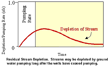 The examples (in the "Response Functions- What are They?") illustrated how response functions can be developed and used when wells are operating continuously. In reality, however, this is seldom the case. We need to be able to evaluate stream depletion from wells that are used intermittently. Response functions can be determined for wells that are pumped for a brief period and then turned off. The procedure is described in the section "How are Response Functions Determined?".
Wells that are pumped for a brief period may produce very minor stream depletion effects that persist long after pumping has ceased. The accompanying graph shows that pumping at a rate of 1 cfs has greatly attenuated effects on a hydraulically connected stream reach. Although the illustration is hypothetical, it is important to recognize that ground water pumping impacts may persist for years or even decades into the future, depending upon the scale and properties of the system.
Response Functions & Aquifer Recharge
Most of the above discussion and examples related to depletion of streams resulting from aquifer pumping. In conditions where response functions can be used, pumping and aquifer recharge create equal but opposite effects on stream and spring discharge. Where ground water pumping results in a depletion of surface water resources, aquifer recharge will result in an increase in flows. The rate of increase will be proportional to the rate of recharge.
In the second example, if the well were recharging at a rate of 2 cfs, rather than pumping, then the stream gains would have increased, rather than decreased, by 1 cfs (the response ratio was 0.5) after 100 days.
Combinations of pumping and recharge can be evaluated by adding responses from individual activities on the stream reach of interest.
Response Functions - How Can Response Functions be Used?
Response functions describe the response of specific river reaches to ground water pumping or recharge at specific locations for specific times. In physical situations where response functions are applicable, response functions may have several uses.
One of the most basic uses of response functions may be to obtain and convey a better understanding of the way in which surface water systems interact with ground water systems. Graphs showing how response (stream depletion) changes with time are one way of gaining an understanding of the attenuation of pumping effects on surface water resources. Superimposing these graphs on a map provides additional information on how impacts change depending on the location of pumping (see figure right). Contouring response ratios (response functions at a single point in time) for an entire aquifer can portray how different pumping locations impact a given river reach. In the Snake River Plain aquifer, contours of steady state response functions (response after many years of continuous pumping) can provide guidance to water managers as to the degree that pumping in any area impacts different reaches of the Snake River: Upper Snake reaches, Blackfoot to Neeley reach, Neeley to Minidoka reach, and Kimberly to King Hill reach.
In many states, ground water and surface water supplies are being conjunctively managed. This integrated management philosophy may result in ground water users being held partially responsible for surface water shortages. If this is the case, then the quantities that individuals or groups of ground water users are accountable for must be determined. This determination is an essential step in development of mitigation plans. Mitigation in the form of managed recharge will be designed to offset injury resulting from pumping. Just as pumping impacts may be readily determined from response functions, the counter-effect of recharge may be assessed. Response functions may be incorporated into spreadsheet water accounting programs to determine debits, credits, and balances associated with ground water pumping and recharge.
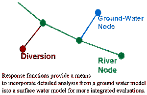 In a simple analytical expression, or a table of numbers, response functions can describe the response of a surface water body to ground water pumping or recharge at a selected location. Subdividing an aquifer into a series of zones allows representation of cause and effect relationships by a simple series of independent equations or tables. These simplified relationships can then be incorporated into regional surface water or multi-disciplinary models that represent the aquifer as one component of a larger system (see figure below). This allows the inclusion of ground water systems into more holistic ecosystem models.
The additive nature of response functions also makes them applicable to optimization techniques. Optimization methods may be used to identify schemes to accomplish goals such as minimizing pumping cost or drawdown at specific locations. Development of response functions is a necessary part of optimization in ground water systems.
Response Functions - How are Response Functions Determined?
Response functions may be determined by several methods. The methods may be divided into three basic categories: 1) direct measurement, 2) analytical methods, and 3) numerical methods. These methods vary in the level of assumtions employed and accuracy of the results. The method selected should be commensurate with the purpose of the evaluation and the information available for each situation. Each method is described in the following paragraphs.
Direct measurement of stream or spring depletion by pumping is possible in relatively few cases. Measurement of depletion resulting from pumping of a specific well is possible only when the well is relatively close to the stream or spring and well pumping is a significant proportion of the stream or spring flow. It is also sometimes difficult to isolate the effects of a single well from other influences that may be causing changes in discharge. When it is possible to measure the relationships between pumping and stream or spring discharge, the proportion of depletion can be determined from measurements of stream or spring flow and well discharge. The depletion changes with time, so observations are required at different times. The response function can be represented by the proportion of well pumping appearing as depletion of the stream or spring. The response function will be valid within some limits of pumping rate, stream flow, and aquifer water level. These limits are site-specific and related to the assumptions identified in the section "Assumptions Supporting Response Functions".
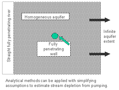 Analytical methods have been developed and used to estimate the effects of ground water pumping on stream depletion. Methods such as those of Jenkins (1968) and Glover (1968) are burdened with intensive assumptions such as straight and fully penetrating streams, fully penetrating wells, and homogeneous and infinite aquifers. These methods, however, can be employed to develop response functions when data are inadequate to use more sophisticated techniques. In these cases, response functions involve little more than plugging the site-specific data into explicit equations.
Response functions can be developed from numerical models in situations where more data are available and numerical models have been developed. Some model codes generate response functions directly, in other situations it may be necessary to run multiple simulations, each simulating response to ground water pumping at a specific location. MODFLOW is the most widely used code for ground water modeling. It is accepted as the industry standard for numerical modeling of ground water systems. Simulated changes, when divided by the magnitude of the pumping rate, yield response functions. The simulations must be based on linear equations. This means that changes in aquifer thickness from pumping must be small relative to total thickness, and head-dependent boundary conditions must be linear functions of aquifer head. This is perhaps the most restrictive condition relative to the use of response functions. If springs dry up, streams transition between hydraulically connected and perched, or other non-linear conditions develop, and if these features significantly affect the operation of the system, then response functions should not be used. Their use should be limited to the range of conditions where these sort of changes do not significantly impact the system. This topic is also addressed in the section "Assumptions Supporting Response Functions".
Regardless of the technique used to develop the response functions, it must be recognized that the response functions are only as good as our conceptual understanding of the system and the data used in the development of the models!
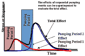 Response functions describe the changes in the system (ground water levels or stream and spring discharge) resulting from ground water pumping or recharge at a specified site for a specified time duration. The response functions become useful tools because of the ability to the add effects of multiple pumping or recharge events. The events may be occurring at the same location sequentially, at multiple locations simultaneously, or both. This makes it most effective to generate response functions for the shortest duration of pumping that is of interest. The response to longer periods of pumping can then be developed by adding the effects from one pumping period to that of a second period immediately following the first. These sorts of operations are ideally suited to spreadsheets and data bases.
Response Functions - Assumptions Supporting Response Functions
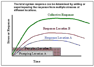 Response functions cannot be universally applied to all situations. The validity of response functions is linked to the concept that responses, such as river depletion from pumping, are additive and proportional to the pumping or recharge rate. This assumption is valid in many ground water environments. Each situation should be evaluated by a qualified professional hydrologist, however, to determine if any of the following excluding conditions are likely to have a significant effect on the ground water flow system in the area of interest.
EXCLUDING CONDITIONS:
1) Saturated aquifer thickness changes, resulting in a significant change in aquifer properties, normally transmissivity.
2) Springs either begin or cease flowing as a result of natural or man-imposed changes in aquifer water level.
3) Streams transition between perched and hydraulically connected with the aquifer.
4) Evapotranspiration or other water consumption varies non-linearly with aquifer head.
5) Enough water is flowing in the river to meet demands in losing reaches.
These conditions need to be evaluated, not just for the development of response functions, but for their application to each specific circumstance. If ground water elevations are changing dramatically in a given situation, then the above conditions are more likely to occur, and response functions should not be used.
Response functions generated by field measurements, analytical techniques, or numerical models will be burdened with all of the assumptions of the method used in their development. For example, if the Jenkins (1968) analytical technique is used to generate the response functions, then one of the assumptions underlying the response functions is that the stream is straight and fully penetrating. If a numerical model is used to generate the response functions, then the accuracy of the response functions is directly dependent on the accuracy of the numerical model's calibration and the underlying conceptual model. In many cases, this will be the greatest source of error in application of response functions.
Hydrologic Unit Codes
H.U.C. is an acronym for Hydrologic Unit Codes. Hydrologic unit codes are a way of identifying all of the drainage basins in the United States in a nested arrangment from largest (Regions) to smallest (Cataloging Units). A drainage basin is an area or region of land that catches precipitation that falls within that area, and funnels it to a particular creek, stream, river and so on, until the water drains into an ocean. A drainage divide is the division between adjacent drainage basins. Just as a creek or stream drains into a larger river, a drainage basin is nearly always part of a larger drainage basin. Drainage basins come in all shapes and sizes, with some only covering an area of a few acres while others are thousands of square miles across. Drainage basins cross artificial boundaries such as county, state, and international borders. The term watershed is often used in place of drainage basin.
Drainage basins in the United States have been divided and sub-divided at four different levels and each assigned a unique hydrologic unit code (HUC) consisting of eight digits based on these four levels. The four levels from largest to smallest are regions, sub-regions, accounting units, and cataloging units.
The first level of classification divides the nation into 21 major geographic areas. These geographic areas contain either the drainage area of a major river, such as the Missouri region, or the combined drainage areas of a series of rivers, such as the Texas-Gulf region, which includes a number of rivers draining into the Gulf of Mexico. Eighteen of the regions occupy the land area of the conterminous United States. Alaska is region 19, the Hawaii Islands region 20, and Puerto Rico and other outlying Caribbean areas are region 21.
The second level of classification divides the 21 regions into 222 subregions. A subregion includes the area drained by a river system, a reach of a river and its tributaries in that reach, a closed basin(s), or a group of streams forming a coastal drainage area.
The third level of classification subdivides many of the subregions into accounting units. These 352 hydrologic accounting units nest within, or are equivalent to, the subregions.
The fourth level of classification is the cataloging unit, the smallest element in the hierarchy of hydrologic units. [Efforts are underway to add further levels of subdivisions.] A cataloging unit is a geographic area representing part of or all of a surface drainage basin, a combination of drainage basins, or a distinct hydrologic feature. These units subdivide the subregions and accounting units into smaller areas. There are 2150 cataloging units in the nation. Cataloging units are the equivalent of a drainage basin or "watersheds".
An eight-digit code (17040206) uniquely identifies each of the four levels of classification within four two-digit fields. The first two digits identify the water-resources region; the first four digits identify the sub-region; the first six digits identify the accounting unit, and the addition of two more digits for the cataloging unit completes the eight-digit code. An example is given here using hydrologic unit code (HUC) 17040206 for the American Falls area. A double 00 in the two-digit accounting unit field indicates that the accounting unit and the sub-region are the same. Likewise, if the cataloging unit field is 00, it is the same as the accounting unit.
In addition to hydrologic unit codes, each hydrologic unit has been assigned a name corresponding to the principal hydrologic feature(s) within the unit. In the absence of such features, the assigned name may reflect a cultural or political feature within the unit. All regions and sub-regions are uniquely named; however, the accounting units are uniquely named only within each region, and the cataloging units are uniquely named only within each accounting unit. Duplication of some names at the cataloging unit level is unavoidable because a large number of streams found throughout the nation share the same names.
Hydrologic unit codes were initiated by the U.S. Geological Survey's Office of Water Data in the fall of 1972 in cooperation with the U.S. Water Resources Council and supported by the U.S. Geological Survey's Resources and Land Information program. Before the HUC system was initiated drainage basins were divided and coded using various methods depending on the organization using them. The HUC codes have created a unifed system between agencies and water-resource planners. These maps, published at a scale of 1:500,000 (1 inch equals nearly 8 miles), present twice the detail of previous river basin maps.
The HUC maps have created a standard for the data collection, storage, and manipulation of files associated with particular river basins.drainage divided. The Geological Survey is using the coding system to document all its water-data collection activities and its data-planning efforts. The Survey's National Water Data Exchange (NAWDEX) system has incorporated the code into its computer system to allow all its members easier access to data holdings that consist of more than a billion water-resource measurements. Other Federal agencies, state county, and city governments are using the HUC's (hydrologic units codes) for coding and managing the data that is collected locally and nationwide.
The Bonneville Flood was one of these ancient catastrophic floods that occurred approximately 14,500 yrs. ago, the result of catastrophic failure of one of the natural dams at Red Rock Pass of Pleistocene Lake Bonneville.
Pleistocene Lake Bonneville covered most of Utah and parts of Idaho and is estimated to have been over twelve times greater in size than the modern Great Salt Lake. When the dam broke, the flood waters involving approximately 4,750 km3 of water, traveled at an estimated 45 miles/hour, carrying 935,000 yds3 of water/sec. eroding the Snake River Canyon to over 500 ft. deep and over a mile wide in some places.
This catastrophic event changed the landscape of the Snake River Plain to what we visibly see today. Several geologic features that resulted from this spectacular event including large bar complexes, fine-grained slack water deposits, scoured and eroded basalt and scabland topography are visible along the flood route.
 Lake Bonneville was the precursor of the Great Salt Lake. The shorelines of this ancient lake can be seen on the higher slopes of the Wasatch Mountains, more than 984 feet above the present level of the Great Salt Lake. Before the catastrophic Bonneville flood, Lake Bonneville covered an area of more than 19,691 square miles.
Approximately 15,000 years ago Lake Bonneville, a late Pleistocene lake, suddenly discharged an immense volume of water to the north. This flood is thought to be caused by capture of the Bear River which greatly increased the supply of water to the Bonneville Basin. These flood waters flowed over Red Rock Pass in southeastern Idaho and continued westward across the Snake River Plain generally following the path of the present Snake River. Although this enormous flood was first described in the literature by Gilbert in 1878, Harold Malde (1968) of the U.S. Geological Survey published the first detailed account of the effects of the flood on the Snake River Plain. The name "Bonneville Flood" first appeared in the literature in 1965 (Richmond and others, 1965).
Large rounded boulders of basalt characterize many deposits left by the flood along the Snake River Plain. H. A. Powers, who recognized that these boulders were of catastrophic origin, and Malde applied the name of Melon Gravel to the boulder deposits (Malde and Powers, 1962). They were inspired to use this term after observing a road sign in 1955 that called the boulders "petrified watermelons."
Release of Flood Near Red Rock Pass
The flood left a ground record of its effects in the Snake River Plain by a variety of depositional and erosional features. At Portneuf Narrows, a canyon 45 miles northwest of Red Rock Pass, the flood is estimated to have reached a height of 400 feet.
The release of water from Lake Bonneville was apparently initiated by sudden erosion of unconsolidated material on the northern shoreline near Red Rock Pass. Although Malde (1968) originally proposed a flood date of approximately 30,000 years ago, he has subsequently revised this age to 15,000 years ago.
Size of the Flood
Malde (1968) estimated that the probable peak discharge of the flood was approximately one-third cubic miles per hour (15 million cubic feet per second). This is to be compared with a maximum historic discharge in the upper Snake River of 72,000 cfs at Idaho Falls in June of 1894. The total flood volume is believed to be about 380 cubic miles.
The catastrophic flood from glacial Lake Missoula, which swept across northern Idaho, Washington and Oregon, caused far more disturbance than did the Bonneville Flood. When the ice dam failed that contained impounded Lake Missoula, 500 cubic miles of water were suddenly released. This flood escaped at a peak discharge estimated to be 9.5 cubic miles per hour. This rate exceeds that of the Bonneville Flood by 30 times.
Duration of the Flood
Malde (1968) suggested that most of the important despositional and erosional features of the Bonneville Flood were developed in a few days; however, the Snake River sustained a high rate of flow for more than a year.
Melon Gravels The Melon Gravels deposited by the flood average three feet in diameter, but some well-rounded boulders range up to 10 feet in diameter. These boulders are composed almost entirely of basalt broken from nearby basalt flows. Only several miles of transportation by the flood was sufficient to round the boulders after which they were dumped in unsorted deposits up to 300 feet thick. Melon gravel bars are as much as one mile wide by 1.5 miles long.
Marginal Channels
Many channels were cut by flood waters near the margin of the main channel of the Snake River. These marginal channels were caused by gravel filling the main channel so that the water was diverted along a new channel. The channels, which measure several miles long and 150 feet deep, were abandoned when the flood subsided.
Scabland
Bretz (1923) first used the term "scabland" in reference to the eroded surface of basalt flows scoured by the Spokane Flood. This erosion was caused by glacial floods removing soil and rock from the surface. Scabland erosional features include coulees, dry falls (alcoves) and anastomosing channels distributed in such a manner as to cause a bizarre landscape. The area affected by the flood can readily be established by the presence of scabland. Gigantic dry falls and potholes range up to 120 feet in depth. Minor features on the basalt bedrock exposed to the flood include polished and fluted surfaces that indicate the direction of the flow.
Blue Lakes alcove, Devils Washbowl and Devils Corral are alcoves along the north canyon rim of the Snake River several miles north of Twin Falls. They were caused by flow from the Rupert channel along a 10-mile-wide spillway. The basalt was thought to have eroded these alcoves by cavitation rather than by cascading water alone. These alcoves formed tiered sets of abandoned plunge pools by stripping off basalt layers 25 to 50 feet thick so as to cause a stair-cased profile.
Stratigraphic Relationship between the Bonneville & Spokane Flood
From 20,000 to 16,000 years B. P. (before present), Lake Bonneville rose gradually until it reached the level of an alluvial spillway. The alluvial spillway suddenly collapsed and the water level dropped about 350 feet from the release of about 380 cubic miles of water. The flood is believed to have occurred between 15,000 and 14,000 years ago with the best estimate at about 14,300 years ago (Currey and others, 1983).
The Bonneville flood followed the Snake River Canyon to the Columbia River in Oregon. At several localities such as Tammany Bar near Lewiston, a tributary of the Snake River, deposits of the gigantic floods merged. Deposits from the Spokane Flood were laid by backflood up the Snake River from the easternmost channel of the scabland. The Bonneville flood deposits were placed over about 20 Missoula backfloods or graded flood-laid beds and 21 more Missoula graded beds overlie the Bonneville-flood gravels. Therefore, the Bonneville flood occurred some time in the middle of the 2,000 to 2500 years period during which the 40 plus Missoula floods were released.
This module includes exercises associated with the effects from the Bonneville Flood along the Western Snake River Plain. The Western Snake River Plain (WSNP) is a northwest trending structural basin that is bounded on both sides by high angle normal faults and filled by more than 4 km of sedimentary and volcanic deposits (Wood and Anderson, 1981). Volcanism of the WSNRP began approximately 14 million years ago with the extrusion of rhyolitic lava flows followed by the eruption of ash flow tuffs. The tremendously thick basalt deposits began approximately 12 million years ago from eruptions of shield volcanoes.
Specific features and regions explored in this module include: boulder bar deposits along Walters Bar, scouring near Swan Falls Dam, potholes near Eden and boulder fields near Hagerman. Most of the deposits associated with the Bonneville Flood are easy to recognize in the field due to their immense size and sedimentary structures and the large percentage of basaltic clasts. Bonneville flood sediments can be separated into two genetically distinct classes; bed load and suspended-load (O’Connor, 1993). Bed load, or tractive, sediments consist of clasts that were transported in continual contact with the river bed prior to deposition and suspended-loaded sediments contain clasts that were transported in the water column and supported by flow turbulence.
Bed Load Sediments
Features that consist of bed load sediment are expansion bars, longitudinal bars, point bars, and pendant bars. Tractive sediments were deposited within the main flood water flow regime where water velocities were high. Expansion bars, one of the largest features visible, and the elongate and narrow longitudinal bars were deposited along the wider portions of the flood route. Expansion bars are visible in the Hagerman Valley and at Walters Bar and a typical example of a longitudinal bar is the Initial Point Bar. Other examples occur in the Hagerman Valley. Point bars, for example Swiss Valley Point Bar, were deposited along the insides of channel bends with surfaces that slope toward the main channel. Pendant bars are narrow and sharp crested and are formed from sediment accumulations behind a resistant protrusion in the flow regime. A typical example of a pendant bar can be seen adjacent to White Butte on Walters Bar.
Suspended Load Sediments
Suspended load features consist of eddy and slackwater deposits. Eddy deposits accumulated in areas of reduced flow velocities, near tributary mouths and in gaps within the canyon wall. In these regions recirculation of water occurs leaving behind finer grained - better sorted sediments that exhibit large scale cross-stratification and a variety of bed orientations resulting from the changing flow patterns. The well sorted gravel deposited in chaotic festoon cross stratification north of Walter Bar is an excellent example of one of these eddy deposits. Slackwater deposits consist of fine laminated clay, silt and sand accumulating in low energy regimes such as basins and ponded areas along the flood route. The largest accumulations of the slackwater sediments are between Swan Falls and Farewell Bend.
Origin of the Snake River Plain
The origin of the Snake River Plain is attributed to several geologic processes.
- Migration of the North American continent over a region of high heat flow (plume or hot spot) in the earth's upper mantle resulting in large volumes of volcanic material being erupted. The age of the volcanic events generally progresses from oldest, about 13 million years ago, to the youngest episodes currently ongoing, traversing from west to east across southern Idaho.
- The volcanic complex identified at Yellowstone National Park is interpreted to represent volcanic events that occurred at various locations along the Snake River Plain as the volcanic activity progressed eastward to its present location. The most recent major eruption in Yellowstone occurred approximately 600,000 years ago (Christiansen, 1982).
- In between explosive rhyolitic eruptions, basaltic volcanism flooded the Snake River Plain, burying the older volcanic structures.
- The western Snake River Plain was down-dropped, lowering the basin relative to the surrounding mountains. Subsequently, the western part of the basin was filled with a thick sedimentary section overlying the older basalts (Whitehead, 1986).
The Snake River Plain is divided into Upper (eastern Snake River Plain) and Middle (western Snake River Plain) segments on the basis of geology and hydrology. The eastern Snake River Plain is underlain by volcanic rock (primarily basalt with lesser amounts of rhyolite) and relatively thin layers or lenses of sedimentary material that thin towards the center of the basin. Prolific amounts of water can be withdrawn from the aquifer associated with the eastern Snake River Plain. The repetitive sequence of successive basalt flows that make up the aquifer provide favorable hydrologic conditions for water to easily move through the system. Transmissivity values (a measure of the ability of water to move through a volume of material) associated with the eastern Snake River Plain aquifer are generally one to two orders of magnitude greater than those determined for the aquifers in the western Snake River Plain (Lindholm, 1996).
The western Snake River Plain is underlain by a section of sedimentary material that may be in excess of 5000 feet thick in the central portion of the basin. The generally fine grained nature of the sedimentary material does not allow water to move as freely as observed in the eastern Snake Plain (Newton, 1978).
What is the Snake River Plain Aquifer?
The Snake River Plain north of the Snake River is a remarkable aquifer of great resource and economic significance. It is not a single homogeneous geologic formation. Rather it consists of a volcanic pile of the Quaternary Snake River Group basalts. In eastern Idaho, these basalts may be about 1 mile thick. The individual flows are 20 to 30 feet thick with the upper 3 to 6 feet consisting of a very permeable rubble zone. Interbedded alluvial sediments are also found between many of the flows.
In the eastern Snake River Plain, the Snake River lies near the southern edge of the plain, about 40 to 50 miles southeast of the ranges of central Idaho. The rivers in the ranges north of the plain all disappear into the surface of the Snake River Plain near the mountain front. The Little Lost River is a typical example. For about 100 miles downstream from Milner Dam in the vicinity of Twin Falls an estimated total volume of approximately 200 billion cubic feet of water (1.4 cubic miles) enter the Snake River from gigantic springs on the north side of the canyon. This is the well-known Thousand Springs area.
Groundwater flows to the southwest through the Snake River Plains aquifer which is consistent with the overall tilt to the southwest of the basalt strata. The channel of the Snake River cuts through the aquifer. Consequently the gravity and weight of the water in the basalt layers north of the river drives the huge springs.
The Snake River Basin - Physical Description
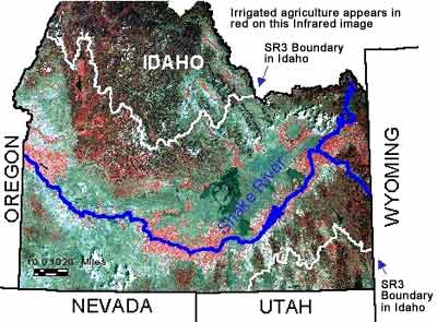 The SR3 study area includes that portion of the Snake River Basin which is upstream of Brownlee Dam. As seen on the adjacent map, the drainage area associated with the Snake River in this study covers portions of five states: Wyoming, Idaho, Utah, Nevada, and Oregon. The Fort Hall (Shoshone-Banock) and the Duck Valley (Shoshone-Paiute) Reservations are also located in the area. The drainage basin includes over 72,000 square miles.
The area includes rugged mountains, semi-arid desert, fertile agricultural land (primarily irrigated), and barren outcrops of lava flows. Most of the famous "Idaho potatoes" are grown in the irrigated portions of the Snake River Plain, but range, lava flows, and timber are the dominant land covers in the basin. Pine and spruce forests inhabit the higher elevations. Most of the land in the basin is owned by the Federal Government (U.S. Forest Service, U.S. Bureau of Land Management, and U.S. Department of Energy).
One of the most prominent physiographic features of the basin is the Snake River Plain. This curved topographic feature extends across southern Idaho into eastern Oregon. The Snake River Plain is approximately 350 miles long and varies in width from 30 to 75 miles. The Plain is discussed in more detail in "Origin of the Snake River Plain" and the "Eastern Snake River Plain".
The Snake River is the dominant hydrologic feature of the basin and is the only river discharging from the area. The Snake extends from its source in Jackson Lake, Wyoming, to its confluence with the Columbia River in Washington. This discussion, however, is limited to the portion above Brownlee Dam. To travel down the Snake River from Jackson Dam to Brownlee Reservoir is a journey of over 700 miles.
Along the way, the Snake and its tributaries tumble over spectacular waterfalls, meander through deep and scenic canyons, and provide the water for irrigating millions of acres of agricultural land.
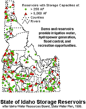 The Snake River is perhaps most well known for its recreational features such as world-class fishing, white water rafting, and the many lakes and reservoirs with excellent opportunities for boating, camping and fishing.
The Snake River has many tributary streams that are important components of the river system. The tributaries provide a means of collecting the precipitation that accumulates in the mountains surrounding the Snake River Plain. Water collected in the tributaries, enters the Snake River directly as surface flows, evaporates, or infiltrates into the subsurface where it later enters the river as spring flows.
Fifteen of the Nation's 65 class one springs (greater than 100 cubic feet per second discharge) are in the Snake River basin. These springs support fish hatcheries that produce the majority of the Nation's commercial trout and produce juvenile fish for planting in lakes and streams.
The amount of natural flow in most of the streams varies throughout the year due to the annual cycle of precipitation. Water accumulates during the winter snowfalls and is released by spring melting of the snow pack. The normally hot dry periods of late summer and early fall are additional factors driving the cyclic nature of flow volumes. In many locations the annual variation in stream flow volume is altered depending on the operational needs of the many reservoirs that have been constructed within the system.
The Snake River and its tributaries, including the aquifers that make up the ground water system, provide water for many uses including: agricultural use, municipalities, industrial and domestic uses, recreation, Native American cultural needs, and habitat for fish and wildlife. The U.S. Bureau of Reclamation, along with other state and federal agencies and private groups, is attempting to manage the water resources of the basin for the many, and sometimes competing, uses. The Snake River Resources Review (SR3) is an effort to take an integrated look at all uses and needs and provide managers with the tools and information necessary to make informed and reasonable decisions. The water resource, and consequently the information, must cross the boundaries of five states and two Indian reservations.
Snake River Plain -Tributary Basins
Basins tributary to the Snake River in the SR3 study area cover parts of Idaho, Wyoming, Utah, Nevada, and Oregon. The Snake River from Jackson Lake, Wyoming to Brownlee Dam, on the Idaho-Oregon border, is nearly 700 miles long. The tributary basins, combined with the east and west parts of the Snake River Plain, drain more than 72,000 square miles (46,000,000 acres). Depending on the scale or detail with which the Snake River drainage system is examined, there are at least 60 separate streams or drainages that connect to the main stem of the river or at least deliver water to the Snake River Plain (Kjelstrom, 1986; Peterson, 1988).
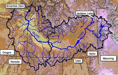 Jackson Lake is the beginning of the Snake River. The lake is nestled at the base of the Teton Mountains within Grand Teton National Park About 15,300 square miles of the study area is associated with the Snake River Plain with an additional 56,000 square miles within the hydrologic units that extend up the tributary basins.
Water in the Snake River begins its journey flowing south through Jackson Hole, as shown in photo to left.. The major tributaries in this region include the Gros Ventre River, Hoback River, Greys River, and the Salt River.
More than twenty tributary streams feed into the Snake River in the eastern portion of the Snake River basin. The larger tributaries in this area include: Henrys Fork, Teton River, Falls River, Big Wood River, Blackfoot River, Big Lost River, and Portneuf River. The Snake River drops in elevation from more than 5,015 feet on the eastern side of the plain, to about 2,100 feet on the western edge near Weiser, Idaho.
The most downstream reach for this study, the Middle Snake-Boise sub basin, extends from King Hill to Brownlee Dam and includes the western Snake River Plain. The western Snake River Plain is about 50 miles wide and 145 miles long (Newton, 1991). The major tributaries in this region include: Payette River, Boise River, Weiser River, Owhyee River, Bruneau River, Malheur River, Powder River, and Burnt River.
Snake River Plain -The Importance of Tributary Basins to the Snake River
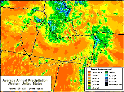 |
|
figure 9. PRISM average annual precipitation map with SR3 outline (after Daly 1998).
Image by Oregon State University. |
While the flow of water within the Snake River receives a tremendous amount of attention, it is necessary to take a closer look at the areas where the flow originates. Precipitation is the sole source of recharge in tributary basins. The Oregon Climate Service (Daly, 1998) created an average annual precipitation map for the Western United States covering the time period 1961-1990 (see map to left). This map shows that within the Snake River Plain precipitation is less than 15 inches per year with some areas receiving less than 10 inches per year. Precipitation totals in the tributary basins can exceed 60 inches per year. These maps were created using the Parameter-Elevation Regressions on Independent Slopes Model (PRISM).
Two factors stand out as reasons to include tributary basins when discussing the flow of water within the Snake River. First, the majority of recharge occurs within the tributary basins. Second, the large areas associated with the tributary basins provide opportunities for development and use of water within the tributary basins themselves. Use of water within a tributary basin can affect the quantity and timing of water availability to the Snake River.
Snake River Basin: River-Tributary Basin Relationships
A basin tributary to the Snake River represents a geographical area with a stream or other body of water, surface or underground, that contributes water to the Snake River, even in small or intermittent quantities. With so many streams and rivers that deliver water to the Snake River, the scale or size of a basin has to be considered in allocating resources for studies or management programs.
Much of the data presented here will use the term “HUCs” (hydrologic unit code), often used synonymously with cataloging units. Cataloging units are the smallest division set aside by the USGS as a system of nomenclature dividing the United States into several large geographic basins or regions that represent hydrologic systems. A cataloging unit may represent a portion of a basin (example- Little Lost), or a combination of drainage basins (example, Upper Snake). In the SR3 study area, there are 53 cataloging units; 26 in the Upper Snake sub basin and 27 in the Middle Snake Sub basin. See illustrations "Eastern & Western" below.
Many different hydrologic relationships could exist between a river and its tributaries. Within the Snake River Basin, three main categories are readily identified:
A. A tributary stream that is not connected to the Snake River.
B. A tributary stream that is connected to the Snake River. Surface water and ground water are not hydraulically interconnected.
C. A tributary stream connected to the Snake River. Surface water and ground water are at least partially interconnected.
Category A-Examples In the northeastern portion of the Snake River Plain, located within the State of Idaho, there are several streams which the Bureau of Reclamation grouped in their SR3 Blueprint (1996) under the heading “Streams that disappear into the Snake Plain Aquifer” (see "Catagory A" figure below). These streams, located on the northern portion of the Upper Snake sub basin, are not tiny ephemeral streams. The largest of the group, the Big Lost River, annually delivers more than 200,000 acre-feet of water that travels down the river to “disappear” or infiltrate into the Snake River Plain. Others in this group include Camas-Beaver Creek, Medicine Lodge Creek, Birch Creek, and Little Lost River. Combined, these basins are the source for over 9 percent (945,000 ac-ft) of the annual water contributions to the Upper Snake River Basin (data from Kjelstrom, 1986).
Category B-Examples: IDWR (Idaho Department of Water Resources, 1997) has described the Rexburg Bench- Moody Creek region as an area that is not hydraulically interconnected with the regional aquifer. In another example, Horn and Jeong (1989), have suggested a similar interpretation describing the Camas Creek basin, Idaho.
Category C-Examples: The third category represents most of the tributary basins. Most of the tributary streams are considered to have at least some degree of interconnectedness with their associated aquifers. It may be difficult in some areas to determine if the associated ground water is the regional system or a perched zone.
Snake River Basin: River-Land Use Data
Recent land use GIS data were obtained from the respective state agencies of Idaho, Wyoming, and Oregon and used to identify presently irrigated lands. Oregon is in the process of converting older data sets to useable GIS files; however, they did provide that portion of the data currently available. There are more areas of agricultural use than shown in Oregon and that data should be available to incorporate into a data set in the near future. Data from Idaho did enable acreage tabulation of the irrigated and non-irrigated lands. See the table below which provides a summary of the distribution of irrigated and non-irrigated acres for HUCs in Idaho.
Teton, Raft, Portneuf, and Blackfoot are those HUCs which contain significant non-irrigated lands with potential for conversion to irrigation. Of the eight HUCs with the largest irrigated acreage, seven are located primarily on the Snake River Plain, see figure below.
|
Basin Name
|
HUC
|
Irrigated Agriculture
|
Non-irrigated Agriculture
|
Total Acres
|
Total Square Miles
|
||
|
Acres
|
Square Miles
|
Acres
|
Square Miles
|
||||
| UPPER SNAKE-ROCK |
17040212
|
820, 645
|
1,282
|
16,325
|
26
|
836,969
|
1,307
|
| AMERICAN FALLS |
17040206
|
692,858
|
1,082
|
182,627
|
285
|
875,485
|
1,368
|
| LAKE WALCOTT |
17040209
|
502,445
|
785
|
214,971
|
336
|
717,417
|
1,121
|
| LOWER BOISE |
17050114
|
472 ,309
|
738
|
9,230
|
14
|
481,539
|
752
|
| IDAHO FALLS |
17040201
|
426,891
|
667
|
67, 520
|
105
|
494,411
|
772
|
| TETON |
17040204
|
333,784
|
521
|
67,774
|
106
|
401,558
|
627
|
| MIDDLE SNAKE-SUCCOR |
17050103
|
269,442
|
421
|
856
|
1
|
270,298
|
422
|
| C. J, STRIKE RESERVOIR |
17050101
|
232,809
|
364
|
20,124
|
31
|
252,933
|
395
|
| LOWER HENRYS |
17040203
|
182,185
|
285
|
182,185
|
285
|
||
| LITTLE WOOD |
17040221
|
170,745
|
267
|
170,745
|
267
|
||
| MEDICINE LODGE |
17040215
|
161,979
|
253
|
161,979
|
253
|
||
| CAMAS |
17040220
|
155,545
|
243
|
150,545
|
243
|
||
| RAFT |
17040210
|
155,020
|
242
|
97,321
|
152
|
252,341
|
394
|
| PORTNEUF |
17040208
|
130,687
|
204
|
234,609
|
367
|
365,296
|
571
|
| BIG WOOD |
17040219
|
129,927
|
203
|
129,927
|
203
|
||
| PAYETTE |
17050122
|
127,203
|
199
|
127,422
|
199
|
||
| BIG LOST |
17040218
|
122,620
|
192
|
122,620
|
192
|
||
| GOOSE |
17040211
|
114,192
|
178
|
114,192
|
178
|
||
| BLACKFOOT |
17040207
|
104,811
|
164
|
22,630
|
35
|
127,442
|
199
|
| N. FORK PAYETTE |
17050123
|
100,157
|
157
|
100,755
|
157
|
||
| WEISER |
17050124
|
86,460
|
135
|
86,460
|
135
|
||
| BEAVER-CAMAS |
17040214
|
85, 826
|
134
|
85, 826
|
134
|
||
| BRUNEAU |
17050102
|
53,184
|
99
|
63,184
|
99
|
||
| MIDDLE SNAKE-PAYETTE |
17050115
|
51,294
|
80
|
51,294
|
80
|
||
| UPPER HENRY'S |
17040202
|
45,700
|
71
|
45,700
|
71
|
||
| SALMON FALLS |
17040213
|
38,878
|
61
|
38,878
|
61
|
||
| UPPER OWYHEE |
17050104
|
35,823
|
56
|
35,823
|
58
|
||
| LITTLE LOST |
17040217
|
34 ,572
|
54
|
34,572
|
54
|
||
| PALISADES |
17040104
|
23,051
|
36
|
65,556
|
102
|
88,607
|
138
|
| S. FORK BOISE |
17050113
|
17,907
|
28
|
17,907
|
28
|
||
| JORDAN |
17050106
|
16,995
|
27
|
16,995
|
27
|
||
| BROWNLEE RESERVOIR |
17050201
|
14,447
|
23
|
14,447
|
23
|
||
| BIRCH |
17040216
|
10,163
|
16
|
10,163
|
16
|
||
| MIDDLE OWYHEE |
17050107
|
7,474
|
12
|
7,474
|
12
|
||
| MIDDLE FORK PAYETTE |
17050121
|
4,839
|
8
|
4,839
|
8
|
||
| SALT |
17040105
|
3,587
|
6
|
3,587
|
6
|
||
| WILLOW |
17040205
|
2,071
|
3
|
117,512
|
184
|
119,643
|
187
|
| S. FORK PAYETTE |
17050120
|
1,047
|
2
|
1,047
|
2
|
||
| S. FORK OWYHEE |
17050105
|
873
|
1
|
873
|
1
|
||
| E. LITTLE OWYHEE |
17050106
|
654
|
1
|
654
|
1
|
||
| LOWER OWYHEE |
17050110
|
135
|
0
|
135
|
0
|
||
| BOISE-MORES |
17050112
|
74
|
0
|
74
|
0
|
||
| N.& MIDDLE FORK BOISE |
17050111
|
||||||
|
Total:
|
5,951,908
|
9,298
|
1,117,114
|
1,745
|
7, 069,022
|
11, 043
|
|
Snake River Basin: Stream Flow Data
Most tributary streams are considered to be at least somewhat hydraulically interconnected with the aquifer, changes in stream flow can affect the amount of water available for aquifer recharge. Also, significant changes in the quantity of ground water diverted or the amount of surface water consumptively used might be indicated by a reduction in stream flow relative to other nearby tributaries. See following table for a summary of stream flows in the Snake River Basin.
|
Table 7. Comparisons of mean annual discharge, Kjelstrom 1986 and 1980 to 1996.
|
||||
|
Update of stream flow data from 1981 to 1996 (Mean annual discharge in thousands of acre-feet.)
|
||||
|
Kjelstrom
|
This study
|
|||
|
Gaging station
|
Stream /Area description
|
Mean for period
of record |
Mean or adjusted
mean for 1934-80 period |
Mean for current
study 1980-96 |
| 13037500 | Snake River near Heise |
5,024
|
4,953
|
5,067
|
| 13046000 | Henry's Fork near Ashton |
1,054
|
1,072
|
1,218
|
| 13047500 | Falls River near Squirrel |
562
|
570
|
544
|
| 13055000 | Teton River near St. Anthony |
586
|
584
|
643
|
| 13055319 | Moody Creek near Rexburg |
11
|
10
|
21
|
| 13058000 | Willow Creek near Ririe |
126
|
126
|
66
|
| 13066000 | Blackfoot River near Shelley |
253
|
253
|
276
|
| 13075500 | Portneuf River near Pocatello |
194
|
193
|
228
|
| 13077650 | Rock Creek near American Falls |
24
|
17
|
23
|
| 13082500 | Goose Creek above Trapper Creek near Oakley |
34
|
33
|
33
|
| 13113000 | Beaver Creek near Spencer (current 4/85-9/93) |
31
|
31
|
15
|
| 13119000 | Little Lost River near Howe (current 4/85-9/90) |
55
|
52
|
57
|
| 131217000 | Big Lost River near Mackay |
219
|
228
|
240
|
| 13148500 | Little Wood River near Carey |
109
|
114
|
118
|
| 13150430 | Silver Creek at Sportsman Access near Picabo |
123
|
140
|
107
|
| 13 l42500 | Big Wood River below Magic Reservoir near Richfield |
332
|
352
|
356
|
| 13154500 | Snake River at King Hill |
7,788
|
7,571
|
7,812
|
| 13168500 | Bruneau River near Hot Spring |
286
|
297
|
269
|
| 13169500 | Big Jacks Crock near Bruneau |
3
|
3
|
5
|
|
Totals:
|
16,814
|
18,533
|
19,078
|
|
Eastern Snake River Plain- Physical Description
 The eastern Snake River Plain extends as a two hundred mile long arc, about 60 miles in width, across southeast Idaho. This plain was formed by the deposition of basaltic lava extruded from numerous vents across the plain. Wind and water deposited sediments overlie the basalt in most areas and are also found interbedded with basalt flows in the subsurface.
Precipitation ranges from about 8 inches/year in the lower elevations in the west to about 14 inches/year in the higher elevations in the northeast. The majority of the water supply originates in mountains on the north and east sides of the basin, including the southern portion of Yellowstone National Park. Within the boundaries of the Snake River Plain, rainfall is insufficient to support commercial levels of agriculture without irrigation that requires substantial diversions from surface and ground-water systems. The Snake River flows along the southern margin of the plain, fed by tributaries flowing out of the mountains on the south and east side of the plain. A few tributaries from the northern valleys flow into the Snake River, but many disappear through seepage into the permeable Snake River Plain basalts.
The Eastern Snake River Plain Aquifer
 |
|
figure 1
|
The aquifer beneath the eastern Snake River Plain is perhaps the single-most important aquifer in Idaho. Composed of layered basalt lava flows and some sediment, it covers an area of approximately 10,800 square mile.
Although the total thickness of basalts is estimated to be more than 5,000 feet (figure 1), groundwater flows most rapidly in the upper 300 - 500 feet, which is the most productive portion of the aquifer. Interconnected pore spaces in the rubbly tops of lava flows transmit water very readily, and well yields above 3,000 gallons per minute are not uncommon.
Total ground-water storage in the upper 500 feet of the aquifer is estimated at 200 to 300 million acre-feet, roughly the equivalent of Lake Erie.
 The direction of ground water flow in the upper part of the aquifer is generally from east-northeast to west-southwest.
Human activity has had a tremendous impact on the water balance of this aquifer. About sixty percent of total recharge to the aquifer is derived from irrigation with surface water (figure 2). Most groundwater still leaves the aquifer via springs and seepage losses in two major upper basin reaches, although pumping withdrawals contribute significantly to the aquifer’s total losses.
Irrigation practices have and continue to exert a major influence on water resources of the Eastern Snake River Plain. Prior to 1950, spring discharges (figure 3) and the water table between Kimberly and Bliss rose by 60-70 feet on average during the period 1907-1959, accounting for a cumulative increase of more than 5 % of the aquifer’s total storage.
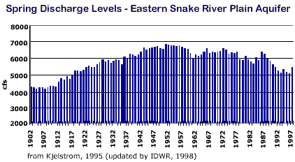 |
|
figure 3
|
During the 1950s and 1960s more land began to be irrigated with groundwater and irrigation efficiency increased through the use of sprinkler irrigation and conservation. The result was a substantial decline in groundwater levels in parts of the Plain between 1975 and 1995, leading to a cumulative decrease in aquifer storage of about 3 %, and decreased spring flows between Kimberley and Bliss (figure 3).
In general, the declines in spring discharge and ground water levels have been due to increased groundwater pumping, more efficient irrigation methods, and reduced reliance on surface water diversions for irrigation. However, localized declines may be predominantly the result of increased pumping withdrawals in some areas.
Eastern Snake River Plain- Hydrogeology
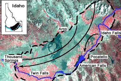 |
| Flow in the Snake River Plain aquifer is generally from recharge areas in the north and east, to springs in the American Falls and Thousand Springs reaches of the Snake River. |
The highly productive Snake River Plain aquifer underlies the eastern Snake River Plain. It has been declared a sole source aquifer by the U.S. Environmental Protection Agency, due to the nearly complete reliance on the aquifer for drinking water supplies in the area.
The aquifer is hosted in layered basalts with sediment occasionally deposited between layers. Highly fractured rubble zones at the contacts between layers provide the primary conduit for ground-water flow. The aquifer is considered to be unconfined but may locally respond as a confined aquifer during short duration pumping. This is presumably due to vertical stratification and the presence of lower permeability sediments interbedded among the basalt layers.
Aquifer recharge occurs mainly in the north and east portions of the plain, resulting in generally southwest trending flow lines. Natural discharge from the aquifer occurs primarily along two reaches of the Snake River: 1) near American Falls Reservoir, in which spring discharges total about 2,600 cfs; and 2) in the Kimberly to King Hill reach (Thousand Springs reach), where the collective discharge is about 5,200 cfs.
During summer, the spring flows provide the majority of the flow in the Snake River below the irrigation diversions of Milner Dam. The Snake River basin contains 15 of the Nation's 65 first magnitude springs (discharge greater than 100 cfs).
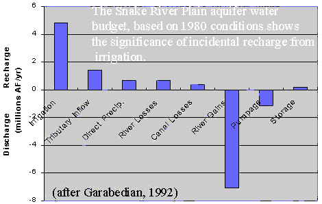 The graph to the left is a water budget for the Snake River Plain aquifer representing 1980 conditions. Surface water irrigation is by far the largest component of aquifer recharge, with smaller contributions from tributary valley underflow and seepage from rivers. During the past several decades, ground water storage has been depleted, causing water levels to drop.
Variations in weather patterns and changes in irrigation practices on the Snake River Plain have caused changes in aquifer water levels. Some areas of the aquifer have experienced drops in water levels where other areas have experienced slight increases in water levels.
One of the major concerns of conjunctive management is the identification of river reaches or surface water bodies that are hydraulically interconnected with an aquifer. The conceptual basis for this concern is described in the section on "Surface Water and Ground Water Interaction". In some cases it is difficult to determine the degree of interconnection because of uncertainties in river bottom conditions and water table depth and because conditions vary with time. A river reach that at one time is hydraulically connected to the aquifer may be perched at another time when aquifer water levels are lower. The State's computer model of the Snake River Plain aquifer treats four major reaches (bounded by gaging stations) of the Snake River as interconnected with the aquifer.
1) The Kimberly to King Hill reach (Thousand Springs reach), in which the river is deeply incised in a canyon and springs discharge along the canyon wall and in the bottom of the river. Total spring discharge in this reach is about 5,200 cfs. The discharge in this reach varies seasonally and also has shown long term variations reflecting weather and irrigation patterns.
2) The Neeley to Minidoka reach which may alternately gain and lose water depending upon water table elevation. The U.S. Geological Survey estimated that this reach had a net gain of 180 cfs in 1980 (Garabedian, 1992).
3) The Blackfoot to Neeley reach in which springs contribute about 2,600 cfs to the flow of the river. Spring discharges in this reach exhibit seasonal variation, but have not shown the long-term variation like the Kimberly to King Hill reach. The reason for the long-term stability in this reach is not known.
4) The Henrys Fork and Upper Snake River reaches which were estimated to jointly gain approximately 260 cfs in 1980 (Garabedian, 1992).
Changes in water table elevation, due to natural causes or man caused activities, result in changes in river gains and losses in these reaches. Although the effects of ground water pumping cannot be measured or separated from effects of natural events, ground water models can provide estimates of individual and collective pumping effects.
Eastern Snake River Plain- Changes in Water Use
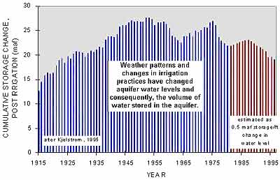 Extensive irrigation from the Snake River and its tributaries began in the late 1800s on the eastern Snake River Plain. Gravity irrigation systems typically divert more than twice the amount of water necessary to meet crop requirements (Goodell, 1985). The remainder of the water returned to the Snake River or infiltrated to the aquifer. The incidental recharge from the approximately 900,000 acres of surface water irrigated land resulted in increased elevation of ground water levels. The volume of water stored in the aquifer, as shown in the above graph, increased by about 15 million acre-feet between 1915 and 1955. On the average, 340,000 acre-feet of water were being added to aquifer storage annually during this period. Spring discharge, especially in the Thousand Springs reach, also increased dramatically during this period due to higher water levels. Cumulative discharge in the Thousand Springs reach increased from about 4,800 cfs in 1915 to about 6,800 cfs in 1955. An infrared image of the plain shows the approximate extent of irrigated lands in the early 1990s for areas that appear in red adjacent to the Snake River.
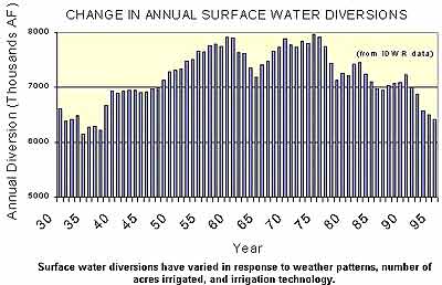 In the mid-1950s, irrigation technology on the eastern Snake River Plain began to change. An increased water use efficiency resulted from completion of additional surface water storage facilities, water conservation programs, and, probably most importantly, increased use of sprinkler irrigation. Surface water diversions for irrigation began decreasing in the early 1970s (see right graph). The increased efficiency of the system led to decreased ground-water recharge that has contributed to the decline of ground water levels and spring discharge. In addition, ground-water withdrawals for irrigation increased dramatically during the last half of the century. About 800,000 acres of ground water irrigated land have been brought into production since the 1950s. At an average estimated irrigation demand of 1.8 acre-feet/acre, the total aquifer withdrawal is about 1.5 million acre-feet/year. The combined effects of decreased recharge from surface water irrigation and increased ground-water withdrawals, along with weather variation, are apparent in the declines in ground-water storage and spring discharge since the mid-1950s. The average rate of decline in ground-water storage between 1975 and 1995 is about 350,000 acre-feet/year.
Eastern Snake River Plain- Recent Challenges in System Management
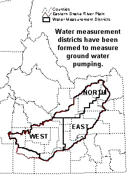 The State of Idaho administers water rights according to the Prior Appropriation Doctrine. Idaho fully recognized the need to implement conjunctive management of its water resources in 1984 when the Idaho Supreme Court determined that hydropower water rights of Idaho Power Company at Swan Falls Dam were not subordinated to junior upstream irrigation rights. The case alerted water users in the basin that ground water pumping for irrigation was impacting spring discharge and flow in the Snake River, and that surface and ground water rights were to be jointly administered. In 1992, a moratorium was imposed on new irrigation pumping on the eastern Snake River Plain (Idaho Department of Water Resources, 1996), which is still in place. Subsequently, IDWR promulgated conjunctive management rules to provide a mechanism to stem conflicts between surface and ground water users when water supplies are limited. IDWR has also formed water measurement districts in the Eastern Snake River Plain (see above figure) that require the measurement and reporting of ground-water pumping at rates exceeding 0.24 cfs, or irrigating areas greater than 5 acres.
Depletion of spring flows and declining ground-water levels are a collective effect of drought, changes in surface-water irrigation acreage and practices, and ground-water pumping. A recent model study (IDWR, 1997) indicates that the collective effects of all ground-water pumping within the boundaries of the eastern Snake River Plain depletes spring discharge and flow of the Snake River by about 900,000 acre-feet per year (1,200 cfs). The same study projects that changes in surface water irrigation practices have depleted the spring discharge by about 500,000 acre-feet per year (700 cfs). IDWR and the courts are placed in the position of determining the degree to which junior ground-water users have injured senior surface-water users. Isolating cause and effect relationships on a case by case basis will be difficult and costly.
Although most water users and managers accept the concept that ground water use depletes surface water supplies, it is not necessarily accepted that depletion constitutes legal injury. The conjunctive management rules provide for weighing the time of year in which depletion is experienced, the efficiency of use of the senior water users, and the maximum economic benefits of all uses, against the possibility of "futile call".
The State's conjunctive management rules allow junior priority water users to mitigate injury to senior surface and ground water users. One of the mechanisms is to provide supplemental recharge to the aquifer. Both surface and ground water users have embraced artificial or managed recharge as a means of avoiding future conflicts and litigation.
Eastern Snake River Plain- Estimates of Surface & Groundwater Interaction
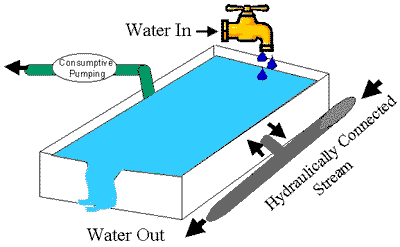 |
|
Aquifer inflows in balance with outflows.
|
There are several reaches of the Snake River, as well as small streams, that are hydraulically connected with the Snake River Plain aquifer. Ground water pumping from the aquifer initially causes a localized decline in the water table. That decline, or cone of depression, propagates progressively outward until it encounters hydraulically connected surface water bodies. The surface water bodies are subsequently depleted as a result of the pumping. There are four primary points to recognize about the effects of pumping on surface water in the eastern Snake River Plain. The reader should recognize that throughout this discussion the focus is on ground water pumping, but the same concepts, in reverse, apply to aquifer recharge.
1) Pumping effects propagate in all directions through the aquifer, not just down-gradient. This means it is possible for a down-gradient water user to affect stream flow in the upper reaches of the plain. This appears to be in contrast to the logic that "water flows downhill", but in fact it is not. Consider the analogy of an water tank in which water is entering from two sources on one end and continuously discharging from an overflow weir on the other end, as shown in the illustration. The water in the tank represents the Snake River Plain aquifer. The one source of fill is a faucet that does not make direct contact with the water level in the tank, therefore it cannot siphon. This represents recharge to the aquifer resulting from perched streams, precipitation, and irrigation sources. If the water level in the tank (i.e. aquifer) changes, it has no effect on this recharge. The second source of fill is a pipe connected below the water surface in the tank. This source represents hydraulically connected stream and river channels. If the water level in the tank drops, more water will flow out of the pipe and into the tank. If a pump is introduced to extract water from the middle of the tank, what will happen? Water levels in the tank will decline, causing the outflow over the weir to be reduced (similar to Thousand Springs). In addition, the inflow from pipe connected beneath the water surface will increase or outflow will decrease (similar to river connection in the Henrys Fork and the upper Snake River). This increase occurs despite the fact that water is flowing through the tank from the inlet to the outlet sides. In the Snake River Plain aquifer, if water is pumped, or recharged, in the center of the plain, gains and losses of the Snake River may be affected at many locations, not just along the flow lines. Flow lines in an aquifer have limited meaning when evaluating the propagation of pumping or recharge effects; they are significant with respect to water quality considerations.
The radial propagation of pumping effects is evident from depletion graphs generated from a numerical model of the Snake River Plain aquifer. It is apparent from the graphs superimposed on the map of the Snake River Plain that effects do not preferentially propagate along the flow lines in the aquifer. Although pumping sites in the upper portion of the basin are aligned with flow lines that discharge near Thousand Springs, the majority of the impact is expected near American Falls. The simulations did not include effects of the hydraulic connection of the Henrys and upper Snake River, although they may be significant.
2) The total volume of water pumped and consumptively used from the Snake River Plain aquifer will ultimately be depleted from surface water sources and cause a reduction in ground water storage. It is obviously true that water pumped and consumptively used is water that would otherwise have gone somewhere else. If we again consider the water tank above, when our pump is taking water out of the tank, the discharge of the tank is diminished and the inflow from the submerged pipe is increased. The pumping has not exceeded the rate of recharge to the tank, but it has impacted outflow (analogous to springs) and inflow (analogous to a hydraulically connected river reach). In the Snake River Plain aquifer, the entire volume of water pumped and consumptively used will either be depleted from spring discharge, cause a corresponding increase in river losses, or cause a corresponding decrease in river gains. We can neither create nor destroy water in the process of pumping.
3) Pumping and aquifer recharge effects on surface water are often greatly attenuated.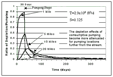 Even though the entire volume of water consumptively pumped throughout the Snake River Plain aquifer will ultimately be drawn from surface water sources and ground water storage, that depletion may be distributed over time periods ranging from days to decades. The attenuation of the effects is related to the proximity of the pumping location and surface water body, and the hydraulic properties of the aquifer and stream. The expected approximate attenuation of pumping or recharge effects within about 25 miles of the Snake River in the Thousand Springs area is illustrated graphically. The effects of a 30 day pumping or recharge event are seen to become more attenuated as the site becomes progressively more distant from the river. The illustration uses aquifer properties typical of the Thousand Springs area that may not be representative of other locations within the Snake River Plain aquifer. At greater distances, the effects are much more attenuated. The effects of a 30 year pumping event in the northeast portion of the plain are expected to continue for decades even after the pumping ceases.
4) Our ability to estimate ground water pumping impacts on surface water resources is limited. 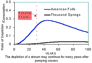 Although this page has presented many illustrations that quantitatively relate consumptive ground water pumping or recharge to surface water depletion, these illustrations are approximate. They are the result of analytical and numerical models, but those models are the current representations of our limited knowledge about the real system. More detail can be found in the section on "Evaluation Methods".
The above points are extremely significant to water management in the Snake River and the Snake River Plain aquifer. Some of the primary management considerations are:
1) Negative impacts can result from consumptive ground water pumping, even though the rate of pumping does not exceed natural recharge. This is because other users or system needs are dependent on the aquifer.
2) There is no "no-impact" consumptive pumping. Every gallon of water consumptively used is not available somewhere else in the system where it would otherwise have existed.
3) Conjunctive administration of water rights under the Prior Appropriation Doctrine will be an involved process. Complication results from the propagation of effects to changes in consumptive ground water pumping or managed recharge in all directions and the attenuation of those effects in the aquifer and to the stream, and due to our limited knowledge about the aquifer.
4) Managed aquifer recharge can offset some of the adverse economic and environmental impacts of consumptive ground water pumping.
Eastern Snake River Plain- Evaluation Methods
Several methods may be applied to estimate the impact of ground water pumping or recharge on surface water resources. General application of these methods is discussed in the section on "Surface Water and Ground Water Interaction". The primary method used for the Snake River Plain aquifer has been numerical modeling. Numerical modeling allows us to use as much information about the system physical characteristics as we have available; however, our knowledge of the system is never complete.
Several models have been constructed of the Snake River Plain aquifer, or portions of the aquifer. The two most complete models were constructed by the University of Idaho for the Idaho Department of Water Resources (IDWR) and the U.S. Geological Survey (USGS). These two models have similar boundaries and employ the same computer code. They differ, however, in their purpose for construction and, consequently, their design. The USGS model was constructed largely as an investigative tool to explore concepts of the regional ground water flow and improve our scientific understanding of the system. The IDWR model was designed primarily as an aquifer planning and management tool. The IDWR model presents a more simplified concept of the aquifer in that it uses a single model layer. The single layer was used because it was felt that data were inadequate to develop the multi-layer approach used by the USGS. Nevertheless, extremely sophisticated concepts can be simulated with each model. Our development of models is limited by data availability and our understanding of the real system. A comparison of predictions from these two models is currently being explored as part of the Bureau of Reclamation's SR3 project. More information on these models can be found in Cosgrove and others (1999) and Garabedian (1992).
The model developed for the IDWR is the tool that has been, and probably will continue to be, used for evaluating ground water and surface water relationships. The model was used to perform the Upper Snake River Basin Study (IDWR, 1997) and was used to develop response functions for the river and aquifer (Johnson and Cosgrove, 1999, to be supplied).
The models of the Snake River Plain aquifer described above have been used for many years and presently are accepted to represent the effects that consumptive ground water pumping and managed recharge have on ground water storage and on interactions between the river and the aquifer. However, it is important to recognize that these models are not precise. Although our models will never be perfect, they can always be improved. For example, more ground water-level measurements are needed near the Snake River to better understand and represent the interconnection between the river and the aquifer.
Western Snake River Plain- Treasure Valley General Description
 The Treasure Valley, which includes the lower Boise River basin and extends south to the Snake River is located within the northwest-trending topographic depression known as the western Snake River Plain. The western Snake River Plain is a relatively flat lowland separating Cretaceous-age granitic mountains of west-central Idaho from the granitic/volcanic Owhyee mountains in southwestern Idaho. The western Snake River Plain extends from about Twin Falls, Idaho northwestward to Vale, Oregon. The Snake River Plain is about 30 miles wide in the section containing the lower Boise River. The depression is believed to have been formed by crustal extension, beginning as early as 17 million years ago (Malde, 1991).
Western Snake River Plain- Treasure Valley Water Use
 Agricultural
Approximately half of the land in the Treasure Valley is irrigated agriculture, and of this, approximately 74% is irrigated with surface water. Surface irrigation water is distributed through an extensive series of canals. The largest of these, the New York Canal, diverts approximately 2,500 cfs in a typical irrigation season. The canals are operated by a variety of irrigation districts, canal companies, and other entities.
An acre-foot is an expression of water quantity. One acre-foot will cover one acre of ground one foot deep. An acre-foot contains 43,560 cubic feet, 1,233 cubic meters, or 325,829 gallons (U.S.).About 1,380,000 acre feet per year are diverted for agricultural irrigation from the Boise River. In addition, approximately 360,000 acre feet are diverted from the Payette River to the Treasure Valley.
Ground water is used to irrigate approximately 42,300 acres of farmland, primarily in the southern portion of the valley. In addition, many of the irrigators dependent on surface water supplies use supplemental irrigation wells during periods of drought. It is estimated that approximately 72,000 acre feet of ground water are withdrawn annually for agricultural irrigation. The image above shows a typical pivot irrigation system in the Treasure Valley.
Municipal Most municipal water in the Treasure Valley comes from ground water. Municipal water is supplied by a variety of entities, including public companies, cities, and water districts. The Idaho Department of Environmental Quality has compiled a map. The largest water purveyor in the Treasure Valley is United Water Idaho (UWI). UWI provides water services to about 190,000 people in Boise and surrounding communities. The company is a subsidiary of United Water Resources, one of the nation's largest water services companies
United Water Idaho customers receive their water from both groundwater and surface water sources. Groundwater is drawn from wells drilled into deep aquifers that produce about 14 billion gallons of water per year. The groundwater quality is excellent and free from harmful bacterial contamination. As a result, treatment is limited to disinfection with chlorine. Unfortunately, the advantages of excellent bacteria-free groundwater are often accompanied by disadvantages like high iron and manganese content. This is associated with discoloration problems -- some of United Water's groundwater sources have a high iron and manganese content. We are improving these sources with geoscience techniques to screen out water high in these minerals or by adding a phosphate compound to hold these minerals in solution.
Eight percent of United Water Idaho (UWI) water is drawn from the Boise River at the Marden Street Treatment Plant; 89 wells supply , and 92% is pumped from a total of 89 wells scattered throughout the Boise area. The Marden Lane Water Treatment Plant is a conventional filtration plant that produces about 1.8 billion gallons of water per year. Treatment involves filtering to remove particulate matter, followed by disinfection with chlorine to destroy any harmful bacteria. We also adjust the pH to reduce the water's corrosiveness and decrease the possibility of dissolving metals from household plumbing. Some facts from United Water Idaho's website:
|
Source of Supply
|
|
|
Total capacity
|
92 million gallons per day |
|
Water treatment plant
|
1 with a capacity of 16 million gallons/day |
|
Operating wells
|
89 with a capacity of 76 million gallons/day |
|
Average well pumpage
|
650 gallons per minute |
|
Average well depth
|
550 feet |
|
Deepest well
|
1,120 feet |
|
Water Usage in 1999
|
|
| Water delivered | 15.8 billion gallons |
| Average daily usage | 43.2 million gallons |
| Peak usage | 85.5 million gallons |
|
Distribution System
|
|
| System coverage | 160 square miles |
| Pressure Zones | 6 |
| Mains | 845.6 miles |
| Main size | 2 inches to 24 inches |
| Reservoirs | 27 |
| Reservoir Capacity | 31.05 million gallons |
| Booster stations | 38 |
Commercial & Industrial
Industrial ground water use is difficult to quantify because many industries rely on different water sources, such as a combination of municipal supply and self-supplied water.Also, municipal suppliers usually do not distinguish between commercial and industrial use, i.e., the commercial category includes small businesses, multi-family housing, and industrial facilities.That said, the estimated self-supplied industrial ground water withdrawals in 1996 are shown in the table below (Urban and Petrich, 1998).
|
Industry (1)
|
Total Self-Supplied
Industrial Withdrawal |
|
acre-feet/year
|
|
|
Agriculture (3)
|
60 |
|
Construction
|
5,550 |
|
Food Processing
|
9,180 |
|
Manufacturing (4)
|
3,310 |
|
Micron Technology (5)
|
1,690 |
|
Wood Products (6)
|
990 |
|
TOTAL:
|
20,780 |
Notes:
1. Industry categories and 1995 employee census data from Idaho Dept. of Employment, Research and Analysis, except for Micron Technology, Inc, which supplied its own population and water use data for 1995.
3. Agriculture category refers to amount of water personally consumed by the employee; does not include irrigation water, livestock water, or other agricultural uses. Rate of 15 gpd/person obtained from Idaho Water Law Handbook, 1988, Appendix IV; value for "day camps, no lunch served."
4. Manufacturing category includes electronics industries (except Micron Technology, Inc. of Boise, which is considered separately).
5. This rate reflects the amount of water pumped from Micron wells only; an additional 123 gpd/employee was purchased from United Water Idaho.
6. Wood products category includes lumber and wood industries, such as lumber, plywood, and cabinet making. It does not include pulp and paper industries.
Western Snake River Plain- Treasure Valley: The Boise River
The lower Boise River is the 64-mile stretch that flows from Lucky Peak Dam above Boise, Idaho to the Snake River below Parma, Idaho. The river flows primarily through Ada and Canyon Counties, but also drains portions of Elmore, Gem, Payette, and Boise counties. The watershed encompasses 1290 square-miles of rangeland, forests, agricultural lands, and urban areas. The river flows in a northwesterly direction from its origin at Lucky Peak Dam to its confluence with the Snake River.
|
Boise River- Typical July Conditions
|
 |
|
Boise River Diversions
|
 |
Diversions and Returns
The Boise River is the primary channel bringing water to the Treasure Valley, and a primary destination of ground water discharge. Water is withdrawn for the Boise River beginning at Diversion Dam. Some of the water seeps from the Boise River into underlying shallow aquifers, primarily above Capital Street Bridge. Water returns to the Boise River as (1) return flows from irrigation (water that was diverted but not used), (2) ground water discharge to canals (that then flows into the Boise River), and (3) direct ground water discharge to the river channel.
The graphic (right) illustrates flows out of and into the Boise River under typical July conditions. Note that flows may be reduced to 250 cubic feet per second (cfs) in the vicinity of Star Bridge. Below this point return flows exceed diversions.
Flooding
Annual flooding has been reduced substantially since the construction of three major dams in the upper Boise River Basin – Anderson Ranch, Arrowrock, and Lucky Peak. Reservoirs created by these dams reduce flooding in the lower Boise River and store water for use during summer irrigation. However, flooding still occurs, from dam releases under full reservoir conditions and from surface water runoff from tributary basins in the Treasure Valley. The Federal Emergency Management Agency (FEMA) is the independent agency of the federal government responsible for protecting the public when it comes to flooding.
In September of 1999, the Idaho USGS completed a "Restudy of the Boise River Flood Plain in Ada County, Idaho". The USGS surveyed Boise River cross sections and identified existing elevation reference marks. FEMA (Federal Emergency Management Agency) will use this information to update the flood plain and floodway boundaries along a 32 mile stretch of the Boise River from Barber Dam to the Ada/Canyon county line. The Federal Emergency Management Agency -- FEMA -- is an independent agency of the federal government, reporting to the President. Since its founding in 1979, FEMA's mission has been clear:
to reduce loss of life and property and protect our nation's critical infrastructure from all types of hazards through a comprehensive, risk-based, emergency management program of mitigation, preparedness, response and recovery.
Surface Water Quality
Terms such as effluent trading, Total Maximum Daily Loads, and run-off are issues that affect the quality of the Boise River.
The Idaho Department of Environmental Quality has produced a draft document in pdf format called "Lower Boise River Nutrient Subbasin Assessment". It provides an overview of the Lower Boise River Watershed, including characterization, water-quality concerns, pollution-source inventory, and pollution-control efforts as they pertain to nutrients. (pdf 1.1 Mb, 61 pages)
The Idaho Department Of Environmental Quality report, "Summary of Participant Recommendations for an Effluent Trading Framework (Lower Boise River)" summarizes the efforts of the Lower Boise River Effluent Trading Pilot Project participants, and the recommendations that have emerged for an effluent trading program framework.
"Lower Boise River Nutrient Subbasin Assessment" is a draft document which provides an overview of the Lower Boise River Watershed, including characterization, water-quality concerns, pollution-source inventory, and pollution-control efforts as they pertain to nutrients. Public comment period closed August 17, 2001. (pdf 1.1 Mb, 61 pages).
Western Snake River Plain- Treasure Valley Ground Water
|
Conceptual Cross-Section (Regional Scale)
|
 |
Ground Water Flow Systems
The Treasure Valley contains a complex system of shallow, intermediate, and deep aquifers. Shallow aquifers often supply water to rural domestic and some irrigation wells. Municipal, industrial, and some irrigation wells typically draw water from deeper aquifers. Intermediate aquifers, found in the transition from shallow to deep zones, supply water for domestic, irrigation, and municipal uses.
Shallow aquifers, present throughout the central portion of the Treasure Valley are often contained in the Snake River Group sediments. Depths of these aquifers are generally less than 250 feet below ground surface. Ground water in shallow aquifers generally originates at ground surface, in the form of precipitation, infiltration from irrigated areas, or infiltration from river and stream channels or canals (see “Aquifer Recharge”). Shallow aquifers can contain very localized flow systems such as from an irrigated field to the nearest drainage ditch, or extend tens of miles.
A deeper, regional aquifer system underlies shallower aquifers. The regional system extends throughout the valley, with ground water flowing in a generally westerly direction. Water enters the regional system at the basin margins or in the easternmost portions of the valley. Some of the tilted sedimentary zones underlying the geologic unconformity represent productive aquifer zones. Coarse-grained sediments overlying the unconformity may act as a manifold distributing water from the east Boise and/or peripheral areas into the underlying aquifer zones.
|
Estimated Recharge to Shallow Aquifers
|
 |
|
Aquifer Water Balance
|
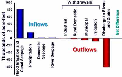 |
Aquifer Recharge
“Aquifer recharge” refers to the water that is entering the aquifer system. Recharge to the Treasure Valley aquifers was estimated on the basis of land use (Urban and Petrich, 1998) . Approximately 50 percent of the Treasure Valley land area is flood or sprinkler irrigated. Seepage from flood irrigation (including canal seepage) accounts for approximately 95 percent of recharge to shallow aquifers. Only a small portion of this water, however, enters deeper aquifers; most of the shallow aquifers discharge into river, canal, or ditch channels.
Infiltration from flood irrigation and canal seepage far exceeds recharge from precipitation or other sources (see “Water balance”). Ground water withdrawals for industrial, rural domestic, municipal, and irrigation uses are much less than the water that returns to ground surface as natural discharge. However, much of the withdrawals occur from deeper aquifer zones, while much of the discharge occurs from shallow aquifers.
References:
Urban, S.M. and Petrich, C.R., 1998. 1996 Water Budget for the Treasure Valley Aquifer System, Idaho Department of Water Resources Research Report.
Ground Water Levels
Ground water levels have been measured on a regular basis as a part of the Treasure Valley Hydrologic Project. Over 350 Treasure Valley wells were measured six times in mass measurements. A mass measurement is the measurement of a large number of wells in a short time (in this case, usually within a one-week period). Mass measurements were conducted in spring and fall of 1996, 1998, and 2000 by the U.S. Geological Survey (http://id.water.usgs.gov/). A mass measurement provides ground water level information at one period in time, which is used to determine a potentiometric surface (in an unconfined aquifer the potentiometric surface is the water table). The potentiometric surface is used to determine ground water flow directions.
In addition, water levels in about 70 wells have been measured on a monthly basis. Hydrographs, drawn from monthly water level data, are a graphic representation of water level data over time for one location.
Ground Water Level Changes
Seasonal changes in ground water levels can range from few to about 10 feet. These seasonal variations depend on the amount and timing of local recharge and pumping.
Ground water levels in most parts of the Treasure Valley have remained relatively constant. A water level change map for the Treasure Valley compares water levels from the period 1969-1976 with water levels in the year 2000.
Treasure Valley ground water quality was documented in 1998 as part of a statewide water quality monitoring program (Neely and Crockett, 1998) . Drinking water aquifers were grouped into two hydrogeologic systems. The shallow system included those aquifers generally less than 250 feet below ground surface, and above the “blue clay". The deep system consists of the aquifers that generally are deeper than about 250 feet and are below the “blue clay”.
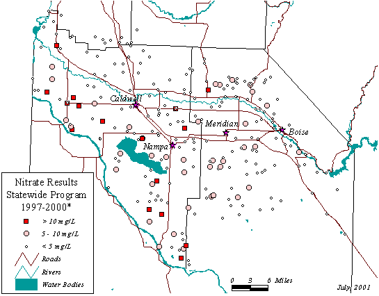
Water quality constituents were analyzed in water samples from 281Treasure Valley wells. The constituents included common ions (calcium magnesium, chloride, sulftate, etc.), nutrients (nitrate, ammonia, etc.), trace elements (arsenic, copper, iron, zinc, etc.), radioactive elements, volatile organic compounds (benzene, perchloroethylene, etc), bacteria, and pesticides.
In 1997, 49 (17 percent) of 281 sampling sites (wells) had one or more constituents with concentrations greater than primary Maximum Contaminant Levels (MCLs) (Neely and Crockett, 1998) . The MCLs are established by the U.S. Environmental Protection Agency (EPA) for public dringing water supplies. Constituents exceeding these standards included arsenic, bacteria, fluoride, nitrate, and some volatile organic compounds.
Nitrate is often an indicator of aquifer vulnerability because higher concentrations are generally caused by land use activities. More recent data collected between 1997 and 2000 show that 35 percent of the Statewide Program wells in the Treasure Valley shallow system had nitrate levels equal to or greater than 5 milligrams per liter, and ten percent had concentrations over 10 mg/l (Neely, 2001) . Nitrate concentrations of two mg/l generally are considered to be above background in the Treasure Valley, and 10 mg/l nitrate is the drinking water standard. The map below shows the distribution of elevated nitrate concentrations in the Treasure Valley. More information on recent water quality measurements is available from http://www.idwr.state.id.us/planpol/techserv/gwmon/status_of_gwq_tv.pdf.
Irrigation in Idaho goes back to small beginnings at least as far as 1839 when Henry Harmon Spalding put in a ditch to save his crops at his Nez Perce mission that summer. Another mission station at Kamiah also needed to try out irrigation that summer. But the beginnings of anything like extensive reclamation of Idaho’s arid lands had to wait another sixteen years. At the Mormon Salmon River Mission on the Lemhi, diversion of the water of Pattee Creek commenced June 27, 1855, and a small ditch dug that year is still in use in the Lemhi Valley. When Mormon settlement in Cache Valley advanced northward to Franklin in 1860, irrigated farming made that new community-Idaho’s oldest town - possible.
As the Mormon settlements expanded into other parts of southeastern Idaho (beginning with Bear Lake Valley in 1863) irrigated farms spread over that part of the territory. Gold discoveries in the Boise Basin in 1862 brought irrigated farming to the nearby valleys the next year. In 1863, all the easily watered lands immediately adjacent to the Boise River were taken up and farmed, and by 1864 some important canal companies were getting started. Many early ditches were extended cooperatively by a group of interested farmers whose organization was informal at best. In order to get water onto more difficult bench lands, extensive capital investment was required for the large canals which had to be engineered and dug. Enterprises of this scale could be managed in the upper Snake River Valley by the Mormons who already were organized for community cooperative action. But in southwestern, Idaho, privately incorporated canal companies began to do the job. The Ridenbaugh Canal is a good example of this kind of construction, and the New York Canal started this way.
Failures of canal companies, not only in Idaho, but over the West in general, to manage large-scale reclamation led to arrangements for state assistance. Under the Desert Land Act of 1894 (generally known as the Carey Act) the President of the United States was authorized to transfer up to one million acres of arid land to each of the reclamation states with public lands; the states then could sell the lands in 160 acre lots to the farmers who would be served by canal companies under arrangements approved by the state reclamation engineer. To qualify for lands under the Carey Act, Idaho immediately established the office of reclamation engineer and provided for the organization of irrigation districts of interested farmers. (Irrigation districts are special districts somewhat like school districts, only providing for reclamation rather than education.) Some years went by before the law was perfected to the point that an irrigation district could be set up under it. But by 1900 the Pioneer Irrigation District was established around Caldwell, and others soon followed. Meanwhile, steps were being taken to irrigate a large tract of land in the Twin Falls country under the Carey Act. By 1905 a large canal from Milner Dam was bringing water onto new farms in the desert lands south of the Snake River, and a few years later, Carey Act lands on the north side were receiving water from Milner.
Idaho benefited from the Carey Act far more than did any other state: about 60 percent of all Carey Act lands irrigated in the United States are in Idaho. Since most of the reclamation states could not manage to use the Carey Act to advantage, another reclamation act of 1902 provided for a United States Reclamation Service (now the Bureau of Reclamation) to work through irrigation districts in the western states. Capital and engineering necessary for great dams and distribution systems were provided from land revenues by the United States on the condition that the irrigation districts repay the costs of their projects. The Minidoka projects around Rupert and Gooding and the Boise Project in southwestern Idaho grew out of the 1902 act. For the Boise area, such enterprises as the New York Canal (which had commenced as a private canal company venture) were brought to completion under federal reclamation ; great new reservoirs and dams--the major early one being Arrowrock, which was highest in the world for about twenty years after its completion in 1915--were added shortly. Later dam construction by the Bureau of Reclamation served major Carey Act, as well as Reclamation Act, projects: American Falls (1927), Cascade (1948), Anderson Ranch (1950), and Palisades (1956), being the more notable.
Unlike most of the western states, Idaho still has successful samples of all four stages of reclamation in operation: scattered individual farmers with their own little ditches and diversions; private canal companies, primarily in the upper Snake River Valley; Carey Act projects, mainly around Twin Falls; and Reclamation projects, the largest of which are Boise and Minidoka. And since 1950 extensive pumping of underground water for irrigation has transformed thousands of acres of land in the Snake River plains which could not be served so easily by canals. Future extension of Idaho’s irrigated farmlands is expected to increase the total amount of reclaimed land very considerably. But in the meantime, a large number of ditches--some of them over a century old--continue to serve countless Idaho farms.Original content compiled by Christian Petrich, Margie Wilkins, Tondee Clark, and Tony Morse.
Photos provided by U.S. Bureau of Reclamation, Idaho State Historical Society, Idaho State Department of Agriculture, Idaho Department of Water Resources.
Adaptation for the Digital Atlas of Idaho by Ean Harker- design/html, Kyle Raverty- content, 11-2002.
Information supplied by the Idaho Department of Water Resources; 1301 North Orchard Street Boise, Idaho 83706 (208) 327-7900.
Thermal Waters
 |
Hot water bubbling out of the ground has been known about and used in Idaho for hundreds, probably thousands of years. Concentrations of artifacts at and petroglyphs on rocks near hot springs are evidence that the areas were known about and used by Indians. More than 200 hot or warm (thermal) springs occur in Idaho and are distributed throughout several geologic provinces. In order for a spring to be classified as thermal it must be at least 68'F (20'C). Some of Idaho's hot springs reach temperatures as high as 200'F (94'C). Even higher temperatures have been encountered in deep wells.
Origin of Hot Springs
Hot springs develop when rain and melted snow waters infiltrate into the ground. This ground water then sinks deep into the earth and is warmed by the heat contained in the earth's interior. Because hot water is less dense it is pushed back to the surface by the continued sinking of heavier, cold water. Annual replenishment to the system by cold meteoric water creates a continuous system which is called hydrothermal convection. Hot springs develop when the upwelling hot water rises along faults or other fractures in the earth's crust and flows out onto the surface.
Sources of Heat
 |
|
Public pools & gardens at
Lava Hot Springs, Idaho |
Why do some areas of the earth have hot springs and others do not? For example, there are few if any hot springs identified in Idaho north of Idaho County. While there is heat in the earth beneath any spot on the surface, this heat is concentrated closer to the surface in some areas. One means of near surface concentration is a shallow magma chamber within the earth's crust such as would exist beneath a volcano. Yellowstone National Park is centered on such a volcano. We know from measuring the way in which the vibrations of distant earthquakes pass through the Yellowstone area that there is a body of molten rock (magma chamber) at a depth of about 3 to 6 miles. The resulting hydrothermal systems are world famous.
Another area where the heat of the earth can be concentrated near enough to the surface to generate hydrothermal systems is where the crust of the earth is stretched and thinner than normal. Such a condition exists over southern Idaho in the Snake River Plain and Great Basin areas. A number of large warm water systems occur in this region of Idaho including the Boise, Twin Falls, Bruneau-Grandview, Raft River and Mountain Home systems.
Hot to warm springs also occur within the rocks of the Idaho Batholith. The heat in the batholith is believed to result from the decay of radioactive elements contained in many of the minerals which commonly occur in the granitic rocks.
Relationship of Faults to Hot Springs
Now that we have our sources of heat, we need a path for getting the hot water to the surface. In an active volcanic area such as Yellowstone, faulting is created by upward pressure exerted by rising magma, by explosive eruptions, and by deflation of a depleted magma chamber after an eruption. The latter mechanism is the most common and forms what is called a ring fracture system which approximates the outline of the magma chamber. Yellowstone has the added advantage of being astride a zone of active northsouth to northwest-trending faults known as the Intermountain Seismic Belt. The broken rocks within the fault zones in Yellowstone act as an excellent conduit for circulating ground water.
The Snake River Plain and Great Basin area of southern Idaho are being stretched. This is a very advantageous geologic situation for the formation of hydrothermal systems because this not only creates a thin crust to bring heat closer to the surface but it also develops numerous normal faults and keeps them relatively open so that water can easily circulate through them.
Hot springs in the batholith are also the result of deep circulation of ground water in fault zones. It appears from recent geologic mapping that some of the normal faults of the Great Basin continue into the batholith. The batholith has also been subjected to other episodes of faulting.
Mineral Deposits
An interesting feature of hot springs is their associated mineral deposits. Yellowstone, for example, contains several types of hot springs deposits, some of which have resulted in spectacular rock formations.
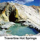 Minerals are more readily dissolved in hot water. The type of minerals deposited depends on the temperature of the water and the type of rocks it passes through on its way to the surface. Mammoth Hot Springs in Yellowstone is a large hot spring deposit of calcium carbonate (calcite).
Table Rock near Boise is a hot spring deposit composed of silica, mostly in the form of chalcedony. At Mammoth Hot Springs the hot water is rising along faults in Paleozoic-age limestone which is composed almost entirely of calcium carbonate. The relationship here is evident. Hot water dissolves the calcium carbonate at depth, transports it to the surface and then redeposits it at the surface as the water cools and loses its ability to keep the minerals in solution.
At Table Rock the hot water passes through mostly volcanic rocks and some sedimentary rocks that have been derived from the granitic rocks of the Idaho Batholith. These types of rocks generally contain about 60 to 70% silica. Once again the relationship is evident. Hot water dissolves the silica out of the rocks and redeposits it near the surface as the water cools and the silica drops out of solution.
Boise Geothermal System
To put our concepts to work and reinforce them let's take a look at an individual system. The Boise system is one of the most studied within Idaho and is generally representative of systems in the southern part of the state. This system is located on the northern margin of the western Snake River Plain graben. The heat source for this area of Idaho is the stretched and relatively thin crust. For reasons that are not well understood the heat in the western Snake River Plain is concentrated along the margins of the Plain. This is fortunate because the faults along which the plain is downdropped also occur along the margin. The main Boise Front fault can be readily seen as a distinct topographic break between the plain and mountains along the north edge of Boise. Comparison of rocks in the foothills of the Boise Front with those encountered in wells drilled in the plain has further confirmed the existence of offset along this fault and in fact has made possible the identification of a series of faults. The water of the Boise system circulates to depth along this series of faults, is heated, and is driven back to the surface by hydrothermal convection. In Boise, springs no longer flow at the surface because wells drilled into the fault zone to tap the hot water have intercepted and withdrawn the hot water rapidly enough that it no longer reaches the surface.
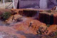 |
|
Hot Springs- Preston, Idaho
|
There is an interesting feature of the Boise system that may explain why it and other systems along the margin of the plain are located where they are. Recent geologic mapping has identified a major northeast-trending fracture system within the Idaho Batholith which appears to extend through the Boise geothermal area. This fracture system provides an excellent channel for the ample meteoric water which falls as rain and snow on the Boise Front to infiltrate into the ground and finally into the high temperature zones along the margin of the Snake River Plain. Further work may make it possible to correlate other fracture systems in the batholith to hot springs along the northern margin of the Snake River Plain and thus explain why hot springs do not occur at regularly-spaced intervals.
Geothermal Energy
In recent years hot spring systems, also known as geothermal systems, have become an important source of alternative energy. In a few rare locations in the world, water in the ground is hot enough to exist as steam. In these instances, wells have been drilled into the heart of the steam zone and the steam is used to operate a steam turbine to generate electricity. Such systems exist at Yellowstone but will not be developed because they are within a National Park. The more common type of geothermal system is the hot water type such as occurs in southern Idaho. Electricity has been experimentally generated in the Raft River area south of Malta but further research and development are needed before commercial operations can begin. Boise boasts the oldest geothermal heating system in the United States. In operation since 1890, the system now serves about 400 homes and is tied in to eight major downtown buildings. Other applications in southern Idaho include the use of warm water for fish farming and greenhouse heating.
Written by Robert E. DeTar, Geologist
Idaho has areas of both substantial and negligible topographic relief due to geographic and geologic features creating rivers, creeks, and lakes. Several major river systems cross Idaho and two large rivers are contained completely within the state. The single most unifying geographical feature is the Snake River which has its source in the mountains of Yellowstone National Park and meanders west to the Oregon border and then north to Hells Canyon, where it joins the Salmon, continuing north to Lewiston, where the Clearwater enters, and heads west to join the Columbia River. The river is more than 1,000 miles long and drains more than 100,000 square miles of country. The Snake River carries 40 million acre-feet of water and drops more than 7,000 feet in elevation by the time it empties into the Columbia River.
The Snake River system contains many canyons along its expanses across Idaho. The Snake runs through a canyon fifty miles long as it enters Idaho from Wyoming. Several rivers, tributaries, flow into the Snake and enter through their own canyons. Blue Lakes Canyon is on the Snake River five miles below Shoshone Falls near the city of Twin Falls. Blue Lakes Canyon contains farmland and a country club along the Snake River almost 500 feet straight down from the desert floor. The Hagerman Valley is another interesting segment of the winding Snake River containing a grand Canyon. This valley is a wide canyon having a high, steep north wall that issues beautiful flowing springs, Thousand Springs. Here, millions of gallons of water gush from the rocky canyon wall cascading into the Snake River. Hydrologists infer that the water source is the Big Lost Sinks where the Big and Little Lost River’s disappear into the lava beds near Arco about 150 miles northeast of Hagerman Valley.
The most well known part of the Snake River Canyon, however, is between Idaho and Oregon. It is Hells Canyon, the Grand Canyon of the Snake, or Seven Devils Canyon. It is 7,900 feet from the bottom of the canyon to the top of Devil Peak. This makes it the deepest gorge in North America. It is about 2,250 feet deeper than the Grand Canyon of the Colorado River in Arizona.
In addition to deep canyon gorges the Snake also has several important waterfalls as a result of sudden regional changes in elevation. These include the spectacular Shoshone Falls which boasts, 212 feet of relief, 52 feet more than Niagara. Other waterfalls in the state include Big Fiddler Creek which has one of the highest falls in Idaho - 600 feet high. It is on the South Fork of the Boise River above Arrow Rock Dam. Moyie Falls is noted for its stone formations which make the water seem to be full of colored glass crystals. It is on the Moyie River near Bonners Ferry. Several towns in Idaho are named after waterfalls: American Falls, Idaho Falls, Post Falls, and Twin Falls.
The untamed and imposing Salmon River - "River of No Return" - winds 425 miles through the mountains of central Idaho, its canyon gorge deeper than the Grand Canyon of the Colorado. It flows through the Sawtooth Wilderness Area and finally joins the Snake about fifty miles south of Lewiston. A spawning stream for pacific salmon, it is one of the longest and most rugged rivers lying wholly within one state.
The Clearwater River, of northern Idaho, is another major river system lying entirely within Idaho’s boundaries. Bitterroot mountain streams feed the Clearwater. The Clearwater was used as a passageway by explorers and trappers, and later by miners and loggers because it was much more tame than its counterpart the Salmon River.
Far to the south is the Bear River, 300 miles long, which originates in Utah's Uinta Mountains, winds back and forth north to Wyoming, back to Utah, back to Wyoming, and then enters Idaho. It moves north (staying south of the tributaries of the Snake) and then back southwest, to where it enters Utah and deposits its water in the Great Salt Lake. Early trappers found beaver along the Bear. The Oregon and California trails entered Idaho with the Bear River and followed it for a considerable distance.
Major rivers in northern Idaho include the Kootenai and Pend Oreille, which flow into the Columbia; the Clark Fork, which flows into Lake Pend Oreille; the Saint Maries, the Saint Joe (St. Joe), and the Coeur d'Alene, which flow into Lake Coeur d'Alene; and the Spokane River which carries the waters of Coeur d'Alene Lake to the Columbia.
The Boise, Payette and Weiser flow into the Snake in southwestern Idaho as it forms the Oregon border, and there are many shorter tributaries of the Snake in southern Idaho.
Idaho has more than 2,000 lakes with names, and thousands of others without names. Some Idaho lakes can't be found on any map! Two of Idaho's northern lakes are said to be among the most beautiful in the world. Lake Coeur d'Alene and Lake Pend Oreille (the largest in the state with a surface area of 180 square miles). Both are large beautiful lakes in Bonner, Kootenai, and Benewah counties. Lake Coeur d'Alene is a popular resort area.
Farther north of Lake Pend Oreille is Priest Lake, early a heavily used trapper area. A few miles south of Pend Oreille is Hayden Lake. Surrounded by forested mountains, all of these lakes are in spectacular settings.
Payette Lake in central Idaho north of Boise is also a significant summer recreation destination. Farther east, in the Sawtooth National Recreation Area, Redfish, Stanley, and Alturas lakes fulfill the same role.
In eastern Idaho, only fifteen miles from Yellowstone, is Henry's Lake, a favorite trapper hangout and trout fishing lake. Farther south is turquoise Bear Lake, half in Idaho and half in Utah.
Many of Idaho's lakes are actually reservoirs, formed behind the numerous dams on the state's waterways. Dams are constructed to store water for irrigation, to generate hydroelectric power, and to keep flood water from destroying farms and cities. Idaho's rivers have such dams as the Anderson Ranch, Arrow Rock, Lucky Peak, Black Canyon, Dworshak, and many others.
Idaho’s five major cities are located on the Snake or its tributaries. A dozen or more dams were constructed along its course alone to provide affordable irrigation water and hydroelectric power for thousands of farms, homes, and most of Idaho's industries (two-thirds of the population of Idaho live in the fertile Snake River Valley). The Snake River has dams and reservoirs at Palisades, near the Wyoming line, American Falls, Minidoka, Salmon Falls, Brownlee, Oxbow, and Hells Canyon.I
Snake River water that is captured in reservoirs or flows on to the ocean comes, not from rainfall, but from the snow that accumulates on the vast peaks of Idaho's mountains. Shifting sand dunes near St. Anthony, Bruneau, and Weiser reveals the fragile environment of the semiarid Snake River Plain.
Water Rights and Conjunctive Management
Written by the Idaho Water Resource Research Institute, University of Idaho
Introduction:
Part of the importance of surface and ground water interaction lies in water rights systems. Surface and ground water in Idaho and many of the western states are managed under the Prior Appropriation Doctrine (Idaho Department of Water Resources and the National Water Rights Digest). The doctrine generally follows the principle of “first in time is first in right”. That is, a priority is established for water rights that are based on the date that the water was first put to beneficial use. Junior priority rights may be fully or partially curtailed in times of short water supply to ensure that senior appropriators (water right holders) receive their full appropriation (legal share). The Snake River basin includes portions of Wyoming, Idaho, Nevada, Oregon, and Washington. Each of these states applies the Prior Appropriation Doctrine within their respective boundaries. The following discussion focuses on the Eastern Snake River Plain in Idaho due to the significance of ground water and surface water interaction in that area.
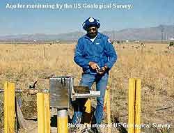 Application of the Prior Appropriation Doctrine to conjunctively managed surface and ground water systems is much more difficult than application to the exclusively surface water systems for which it was initially adopted. Diversion of surface water from a stream impacts downstream users in an amount nearly equal to the rate of diversion, often within a period of a few days or less. Ground water pumping effects propagate through an aquifer in all directions. Ultimately, these effects may reach surface water bodies and result in depletion. Rates of depletion, however, often are less than pumping rates and extended over much longer periods of time. Graphs have been developed illustrating the attenuation of continuous pumping effects in the Snake River Plain aquifer.
Conjunctive Management Rules
In general, surface water rights on the Snake River and tributaries were developed before water rights for irrigation wells. Consequently, ground water pumping rights for irrigation are typically junior to surface water rights. Idaho’s conjunctive management rules hold junior ground water users (excluding domestic use) partially responsible for spring and river depletion that potentially results in injury to senior surface water right holders. Many unanswered questions still exist relative to conjunctive water management in Idaho. These questions include:
1) To what degree does depletion of surface water sources constitute injury to a surface water right holder?
2) To what individual degree are the many ground water users in a basin responsible for a depleted surface water supply?
3) How should depletion rates be determined?
4) How can the prior appropriation doctrine best be applied when the time lags from pumping to depletion effect are so long that curtailing pumping may have no effect on surface water supplies for years in the future?
5) Are junior ground water users responsible for depletion resulting from past pumping practices?
These and other questions are yet to be answered in Idaho. The next decade will no doubt witness significant changes in water management and use in southern Idaho.
Information supplied by Idaho Water Resource Research Institute, University of Idaho December 1998
Authors: Dr. Gary Johnson, Donna Cosgrove, and Mark Lovell.
Photo by US Geological Survey- Dan Ackerman
Graphics: Sherry Laney and Mark Lovell
All State of Idaho images and graphics created with GIS files obtained through Idaho Department of Water Resources Public Domain GIS unless otherwise noted.
What Water Quality Problems are Common in Idaho?
Across Idaho, ground water contamination has been detected in private and public wells. The most prevalent problems arise from nitrates, synthetic organic chemicals, and bacteria.
In a few locations in Idaho, ground water is naturally high in some trace elements such as fluoride. In southwest Idaho, elevated concentrations of arsenic, uranium and sulfate are found in some aquifers.
Non-natural contaminants of greatest potential to impact health in the state are nitrate, volatile organic compounds and pesticides, trace elements (primarily cadmium and selenium), and bacteria. Most sites with elevated nitrate concentrations are in southwest and south-central Idaho. Three percent of all sites tested in the state exceed drinking water standards for nitrate and about one third are elevated through known human influence. The most serious and wide-spread organic chemical contamination occurs in the Boise/Eagle area, around Fort Hall, and in the lower Portneuf River valley around Pocatello and Chubbuck.
Use of MODFLOW for Development of Response Functions
|
Gary S. Johnson and Donna M. Cosgrove
University of Idaho, Idaho Water Resources Research Institute Idaho Falls, Idaho and Joe Spinazola U.S. Bureau of Reclamation, Boise, ID |
PRESENTED AT: MODFLOW '98, GOLDEN, CO., OCTOBER 4-8, 1998, SPONSORED BY THE INTERNATIONAL GROUND WATER MODELING CENTER AND COLORADO SCHOOL OF MINES. |
ABSTRACT
Numerical models, such as MODFLOW, provide excellent tools to assist in the water resourc decision making process. A simplified representation of the system may, in some cases, be obtained by the development of response functions from numerical models. These functions express temporal relationships between cause and effect at specific points within the aquifer and are developed through simulation. The functions are valid so long as the equations governing flow in the system are approximately linear with respect to aquifer head.
. Response functions can be generated from multiple MODFLOW simulations or more simply from the MODFLOW based MODRSP program. Response functions can be developed to describe how aquifer water levels, aquifer storage, surface water depletion, or ground water flow velocities are affected by ground water pumping or recharge in any prescribed location. In areas where the use of response functions is valid, they can provide a highly useful tool for water managers.
INTRODUCTION
Numerical models such as MODFLOW can produce predictive simulations of cause and effect when properly calibrated and applied to an area. This process normally involves comparing results of a series of predictive scenarios to results of a base study, possibly projecting current conditions into the future. The process is valid and useful; however, it requires at least one simulation and comparison for each scenario of interest and has limited capability in presenting cause and effect relationships in more general terms.
Response functions are analytical expressions, graphs, or coefficients that describe the relative response of the aquifer system at a given location to a unit stress at a second location (figure 1, below). Because the response is expressed in relative terms, it may be scaled to any magnitude of stress desired. The functions may express transient or steady-state response of the system to the stress. The development and use of response functions require that response is proportional to the magnitude of the stress; consequently, the governing equations must be approximately linear. Responses may be in terms of aquifer water level change (drawdown), changes in head-dependent flux (capture), change in storage, or changes in ground-water flow velocity. Similar or identical concepts have been called discrete kernels (Morel-Seytoux and Daly, 1975), influence coefficients (Illangasekare and Morel-Seytoux, 1982), algebraic technologic functions (Maddock, 1972) and "drawdown simulations" (Anderson and Woessner, 1992). The assumption of linearity of the governing equations is the major constraint of the application of response functions and will be addressed in greater detail in the following section.
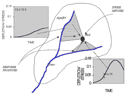 |
|
Figure 1. Concept of Stream Capture Response Functions.
|
There are several ways in which response functions may be applied. They may be used to 1) conceptualize and visualize the manner in which pumping or recharge effects propagate through an aquifer, 2) quantify how aquifer pumping or recharge impacts ground water levels or stream flows, or 3) provide mathematical expressions or matrices to incorporate into more comprehensive water models or optimization schemes. These applications can be accommodated without performing specific predictive modeling scenarios and are described in the following paragraphs.
Response functions can aid in visualization and conceptualization of pumping and recharge effects because the response is assumed to be proportional to the stress. This relationship allows a generic presentation of cause and effect relationships. Hubbell, et al (1997) used a similar approach to describe zones in the Snake River Plain aquifer where ground-water pumping predominantly affects one of four reaches of the Snake River. Refinement of the zones developed by Hubbell, et al (1997) may ultimately form the basis for conjunctive administration of water rights in the eastern Snake River Plain.
Quantification of impacts from individual pumping or recharge activities may be required in adjudication of water rights or development of mitigation plans. Johnson et al (1993) evaluated the depletion of springs from the Snake River Plain aquifer by generating response functions for 18 selected stress locations on the eastern Snake River Plain. The impacts of ground-water use on spring discharge and flow of the Snake River can be approximately assessed for any location on the Plain by using response functions from the nearest location. Similar information may ultimately be used to establish mitigation requirements for ground water pumpers.
The simplified linear form of the response functions permits incorporation into surface water models and optimization schemes. El-Beshri and Labadie (1994) incorporated capture response functions into the surface water model MODSIM (Labadie, 1991). Response or influence coefficients have been applied in simulation/optimization models by several researchers including Ejaz and Peralta (1995).
Response functions can be generated analytically or from calibrated numerical models. Analytically generated response functions are little more than calibration of an analytic expression, such as the Theis Equation, to conditions representing a specific aquifer. Substituting appropriate values for aquifer transmissivity and distance (representing a specific stress location and response location) graphs, response coefficients, or equations can be developed to show how drawdown or stream depletion from a unit stress is related to time. The numerous assumptions inherent in analytical techniques can be avoided by generating response functions from numerical models. The numerical model can be either 1) run under a special set of conditions to evaluate response to a unit stress, or 2) if MODFLOW is used, a special adaptation, MODRSP (Maddock and Lacher, 1991), can be used to generate the response relationships.
The purpose of this paper is to describe how response functions may be generated either directly from a MODFLOW simulation, or through application of MODRSP.
CONSTRAINTS ON USE OF RESPONSE FUNCTIONS
Response functions describe the relative response of the aquifer or stream to an applied aquifer stress. It is normally necessary to assume that the responses of multiple stresses may be superimposed in order to describe aquifer response in general terms. The use of response functions is therefore normally limited to cases where the system can be adequately described using linear equations Reilly, et al (1987) describe the use of linear equations in ground water flow systems.
Numerical models, including MODFLOW, may be based on governing equations that are either linear or non-linear. The partial differential equation representing ground-water flow is linear with respect to the independent variable representing aquifer head. This equation is the foundation from which the finite-difference expressions for saturated, confined, ground-water flow are developed. The linearity of the equation implies that superposition concepts, including response functions, are valid when this equation describes flow within a system.
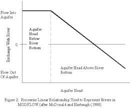 MODFLOW and other numerical model codes include other head-dependent relationships representing system boundaries. Head-dependent functions exist to represent aquifer exchange with rivers, drains, evapotranspiration, and other features. Many of these are represented as piece-wise linear relationships (figure 2). The discontinuity in the linearity of these relationships cannot be accommodated in the use of response functions. The functions will be valid so long as conditions within the aquifer do not cross the discontinuity of slope. When simulating rivers using the River or Streamflow Routing Packages, this is equivalent to requiring that the aquifer heads either continuously remain above or below the elevation of the bottom of the river. The river cannot transition from head-dependent to perched conditions. When simulating drains, the aquifer head at the drain cannot transition across the elevation of the drain. The drain must either remain active or inactive.
Unconfined aquifers require a different form of the partial differential representing ground water flow. The Boussinesq equation is not linear with respect to aquifer head. Superposition and response functions cannot, therefore, be used unless the Dupuit assumption (small head change relative to aquifer thickness) can be applied. If this is not the case, then the response of the system is significantly dependent on other stresses occurring simultaneously, and the system response cannot be expressed without describing all concurrent recharge and discharge activities. Response functions cannot be used in this case.
There are many cases in which non-linearity may exist in a ground-water model. The question to be addressed by the modeler is whether these non-linearities significantly affect the results of the model for the range of stresses of interest. If the non-linearities are negligible, then response functions may be used to approximately describe the response of the system in a general sense. The developer, however, must caution subsequent users of the functions relative to the approximate nature of the functions and the range over which their use is approximately valid.
GENERATING RESPONSE FUNCTIONS USING MODFLOW
MODFLOW can be used in either of two ways to generate response functions. It may be either 1) applied to a single stress with no initial hydraulic gradient, or 2) the user may use the version MODRSP (Maddock and Lacher, 1991) to directly calculate response coefficients. Both methods require the same assumptions and produce equivalent results. Application of MODRSP is normally more convenient than performing multiple MODFLOW simulations; however, MODRSP currently does not include the Drain Package and some of the more recently added modules to MODFLOW and does not include a pre- or post-processor. If newer modules are required for an application, the most efficient procedure may be to conduct multiple MODFLOW simulations.
A calibrated MODFLOW model of an area can be used, with some modification, to directly calculate response functions. Input adaptations are required to remove all recharge and discharge and eliminate all hydraulic gradients within the system. This procedure was outlined and applied by Hubbell et al (1997) and includes the following steps.
- Boundary conditions and stresses are evaluated to ensure they are linear functions.
- Boundary conditions and the spatial distribution of aquifer properties and leakage coefficients are provided by a previous model calibration and/or analytical techniques.
- An arbitrary, horizontal potentiometric surface is established as an initial condition.
- Prescribed head (head-dependent) conditions are established at the same arbitrary datum.
- Unconfined conditions are approximated as confined (when constant thickness can be assumed).
- Recharge and discharge are limited to a single location for a selected point of interest.
If the Drain Package is to be used, the elevation of the drains should be set to the elevation of the starting potentiometric surface and a recharge stress (positive sign) should be applied causing the drain to be active. Altering model input data sets to the described conditions can normally be accomplished within a few hours.
The modified model is run with the single specified stress. System response can be extracted from the model output in either a steady-state or transient form. Development of transient response functions requires that the model include storage characteristics. Response, in terms of changes in aquifer water level, or changes in flux with head-dependent boundaries, can be determined for any desired location by extracting drawdown or flux for that location. In the case of Hubbell et al (1997) the river flux was summed for four reaches of the river and the collective response was described for each river reach. Response to stress at other locations requires repeating the simulation process, again with a single stress used at the point of interest. Hubbell, et al (1997) ran 18 simulations to develop responses for stress at 18 different locations.
An arbitrarily large stress may be used to evaluate the system response. In this case, the stress should be sufficiently large to maintain a reasonably accurate mass balance, minimizing the significance of numerical error. If an arbitrarily large stress is used, the response must be divided by the magnitude of the stress in order to express the results as a response to a unit stress. These results are then easily applied to stresses of any magnitude.
Alternately, a unit stress may be applied at the point of interest. In this case, the iteration closure criteria must be greatly reduced to maintain a valid mass balance and minimize effects of numerical error. The simulated response, however, is produced in a form that is already normalized.
It is also possible to determine the response function as the difference between two simulations where recharge, discharge and hydraulic gradients have not been removed. In this case, the system response at the locations of interest can be expressed as the difference between a simulation with a given stress present and one with the stress absent. The magnitude of the stress, and the closure criteria must be adjusted with consideration of the discussion in the two previous paragraphs.
The second means of obtaining response functions is through application of a MODFLOW variation, MODRSP (Maddock and Lacher, 1991). MODRSP is capable of determining drawdown, velocity, storage loss, and capture response functions. Capture may be stream depletion, change in evapotranspiration, change in head-dependent boundary flux, or leakage from adjacent aquifers. MODRSP is a revision of the 1983 version of the MODFLOW code. Because this program is based on an early version of the program, not all of the currently available packages are accommodated. The SIP, SSOR, and PCG solution packages can be used; however, more recent additions like the Stream-Flow Routing Package are not available. The Drain Package is not included in MODRSP, presumably due to the potential for non-linear effects.
MODRSP solves the finite difference equations for a unit stress for a specified location and duration. Because a unit stress is always used, head change at any location represents the drawdown response function. Capture and storage response functions are calculated from the drawdown response function in the same way as MODFLOW would calculate head-dependent flux or storage change. The velocity response is calculated from inter-cell flow and the equation relating velocity to flow and cell dimensions.
Transient simulations with MODRSP automatically apply a unit stress during the first model stress period. Response functions are provided at the end of each stress period. Response functions generated for subsequent stress periods (after the first) represent the residual effects of the stress through time. Effects of extended pumping may be determined by superimposing response functions with an appropriate time lag.
MODRSP simulates response of the aquifer to a series of stresses at prescribed locations. These stresses are applied through the WELL Package. The user specifies stress locations and MODRSP sequentially simulates individual response to a unit stress at each of the prescribed locations. No other stresses, in the Well Package, Recharge Package, or other packages are input or used. MODRSP automatically applies the previously discussed conditions of no initial hydraulic gradient and no recharge and discharge except at points from which response functions will be evaluated. A personal computer version of MODRSP has been developed in the Civil Engineering Department at Colorado State University.
Either of the two methods described will yield identical response functions. The method chosen should depend on the efficiency of either method for the given situation and the MODFLOW features needed.
ANTICIPATED APPLICATION OF RESPONSE FUNCTIONS IN THE EASTERN SNAKE RIVER PLAIN
The State of Idaho has recently committed to conjunctive management of surface and ground water through the promulgation of conjunctive management rules. These rules focus on the eastern Snake River Plain that contains most of the surface and ground water irrigation in the state. The highly productive Snake River Plain aquifer underlies the eastern Snake River Plain and discharges over 18 million cubic meters per day in the Thousand Springs and American Falls reaches of the Snake River. These spring discharges are highly appropriated for irrigation, hydropower, and other uses. Ground water pumping for irrigation generally has junior water rights priorities relative to the more senior surface water uses. Ground water users are, therefore, likely to be held accountable for depletion of spring discharges and flows of the Snake River.
Although the conjunctive management rules indicate that junior ground water users can be held accountable for depletion of surface water flows, they do not specify a) the rate of accountability, b) how accountability changes with location in the basin, or c) how accountability changes with time. These important details have not yet been determined.
Development of response functions describing cause and effect relationships for different areas of the aquifer and different river reaches may provide a means of understanding and quantifying pumping and recharge impacts on the river. Steady state response functions can be used to identify areas in which pumping most significantly impacts springs along a given reach of the river. Transient response functions will describe the temporal response of spring discharges to ground water pumping or recharge in any given area. It is expected that response functions will be used in a qualitative sense to assist water managers in understanding cause and effect relationships in the aquifer and river and in a quantitative fashion to estimate impacts and mitigation requirements. The U.S. Bureau of Reclamation will also incorporate the response functions into a surface water model of the Snake River.
CONCLUSION
In some cases, response functions can serve as a valuable qualitative tool to aid in understanding cause and effect relationships within an aquifer and as a quantitative tool to express, in simple form, quantitative and transient impacts of ground water pumping and recharge. Response functions can be generated from multiple MODFLOW simulations or more simply from the MODFLOW based MODRSP program. Response functions can be developed to describe how aquifer water levels, aquifer storage, surface water depletion, or ground water flow velocities are affected by ground water pumping or recharge in any prescribed location. The primary constraint on the development and use of response functions is that all significant components of the system must be represented by linear equations. In areas where the use of response functions is valid, they can provide a highly useful tool in a water manager’s toolbox.
ACKNOWLEDGEMENTS
This work is supported by the U.S. Bureau of Reclamation Snake River Resources Review Project (SR3). The work is conducted in collaboration with the Idaho Department of Water Resources.
REFERENCES
Ejaz, M.S. and R.C. Peralta, 1995. Maximizing Conjunctive Use of Surface and Ground Water under Surface Water Quality Constraints. Advances in Water Resources, v. 18, no. 2, pp. 67-75.
El-Beshri, M.Z. and J.W. Labadie, 1994. Optimal Conjunctive Use of Surface and Groundwater Resources in Egypt. Proceedings of the VIII IWRA World Congress on Water Resources, Cairo, Egypt, Nov. 1994.
Hubbell, J.M., C.W. Bishop, G.S. Johnson, and J.G. Lucas, 1997. Numerical Ground-Water Flow Modeling of the Snake River Plain Aquifer Using the Superposition Technique. Ground Water, v. 35, no. 1, pp. 59-66.
Illangasekare, Tissa and H.J. Morel-Seytoux, 1982. Stream-Aquifer Influence Coefficients as Tools for Simulation and Management. Water Resources Research, v.18, no. 1, pp168-176.
Johnson, G.S., C.W. Bishop, J.M. Hubbell, J.G. Lucas, 1993. Simulation of Impacts of Snake River Plain Aquifer Water Use on Flow in the Snake River. Idaho Water Resources Research Institute, University of Idaho, Moscow, ID, 56 p.
Labadie, J.W., 1991. Program MODSIM: River Basin Network Flow Model for the Microcomputer. Dept. of Civil Engr., Colorado State University, Ft. Collins, CO.
Maddock, Thomas III, 1972. Algebraic Technological Function from a Simulation Model. Water Resources Research, v. 8, no. 1, pp129-134.
Maddock, Thomas III and L.J. Lacher, 1991. MODRSP, a Program to Calculate Drawdown, Velocity, Storage, and Capture Response Functions for Multi-Aquifer Systems. Dept. of Hydrology and Water Resources, University of Arizona, Tucson, AZ.
McDonald, M.G. and A.W. Harbaugh, 1988. A Modular Three-Dimensional Finite-Difference Ground-Water Flow Model. U.S. Geological Survey Techniques of Water-Resources Investigations, Book 6, Chapter A1.
Morel-Seytoux, H.J. and C.J. Daly, 1975. A Discrete Kernel Generator for Stream Aquifer Studies. Water Resources Research, v. 11, no. 2, pp. 253-260.
Reilly, T.E., O.L. Franke, and G.D. Bennett, 1987. The Principle of Superposition and its Application in Ground-Water Hydraulics. U.S. Geological Survey Techniques of Water-Resources Investigations, Book 3, Chapter B6, 28 p.